因子分析是指研究从变量群中提取共性因子的统计技术。因子分析可在许多变量中找出隐藏的具有代表性的因子。将相同本质的变量归入一个因子,可减少变量的数目,还可检验变量间关系的假设。
因子分析的原理及具体过程可移步阅读:
本文将基于Python实现因子分析的过程:
# 导入相关包和数据
import numpy as np
import pandas as pd
from factor_analyzer import FactorAnalyzer
from sklearn.datasets import load_breast_cancer
cancer = load_breast_cancer()
import matplotlib.pyplot as plt
import warnings
warnings.filterwarnings("ignore")
# 初始化数据集
df = pd.DataFrame(cancer.data,columns=cancer.feature_names)
df['label'] = cancer.target
df.head()
1 充分性测试
在做因子分析之前, 我们需要先做充分性检测, 就是数据集中是否能找到这些factor, 我们可以使用下面的两种方式进行寻找。
- Bartlett’s Test
- Kaiser-Meyer-Olkin Test
# 载入两个检验
from factor_analyzer.factor_analyzer import calculate_bartlett_sphericity,calculate_kmo
chi_square_value, p_value = calculate_bartlett_sphericity(df)
chi_square_value,p_value

# output
(40197.86999232082, 0.0)
# p-value=0, 表明观察到的相关矩阵不是一个identity matrix.
Kaiser-Meyer-Olkin (KMO) Test measures the suitability of data for factor analysis. It determines the adequacy for each observed variable and for the complete model. KMO estimates the proportion of variance among all the observed variable. Lower proportion id more suitable for factor analysis. KMO values range between 0 and 1. Value of KMO less than 0.6 is considered inadequate.(就是kmo值要大于0.6)
# 导入kmo检验
from factor_analyzer.factor_analyzer import calculate_kmo
kmo_all, kmo_model = calculate_kmo(df)
print(kmo_model)

# outout
0.8431432285264385
# 输出大于0.6故通过检验
2 选择合适的因子个数
在这个问题下, 虽然我们知道了选择5个因子是最合适的, 但是我们也要做一步这个, 正常的时候我们是不会提前知道因子选择的个数的. 我们就是计算相关矩阵的特征值, 接着进行排序.
fa = FactorAnalyzer(25,rotation=None)
fa.fit(df)

ev,v = fa.get_eigenvalues()


# 可视化
# plot横轴是指标个数,纵轴是ev值
# scatter横轴是指标个数,纵轴是ev值

plt.scatter(range(1,df.shape[1]+1),ev)
plt.plot(range(1,df.shape[1]+1),ev)
plt.title('Scree Plot')
plt.xlabel('Factors')
plt.ylabel('Eigenvalue')
plt.grid()
plt.show()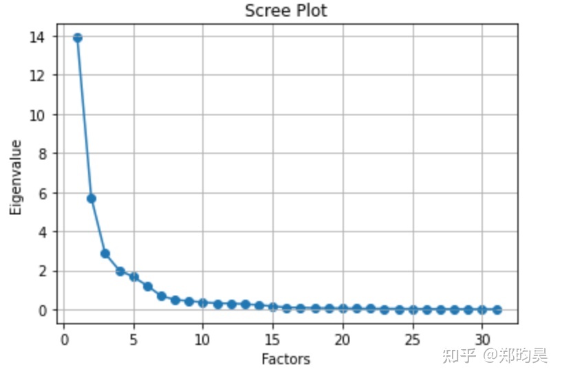

3 因子分析
找5个隐藏因子。
fa = FactorAnalyzer(5, rotation="varimax")
fa.fit(df)

# # 25*5(变量个数*因子个数)
fa.loadings_

# outout
array([[ 0.95398075,  0.04346314,  0.06477682, -0.18221034,  0.09345663],
       [ 0.26037327,  0.01680419,  0.07133274,  0.0679867 ,  0.86155724],
       [ 0.95292205,  0.0822511 ,  0.09996702, -0.16513575,  0.09396329],
       [ 0.96919976,  0.03039574,  0.05984981, -0.10526947,  0.08034304],
       [ 0.190673  ,  0.76998308,  0.06118313,  0.31844238, -0.1303963 ],
       [ 0.46156754,  0.64661612,  0.51645402,  0.08044487,  0.05424249],
       [ 0.6517408 ,  0.44292136,  0.53367333,  0.05217058,  0.09660798],
       [ 0.80474746,  0.43781566,  0.28169349,  0.0382974 ,  0.05916314],
       [ 0.1605024 ,  0.5944214 ,  0.21013331,  0.28649588, -0.01405589],
       [-0.30411784,  0.61510125,  0.47911472,  0.32824546, -0.08585792],
       [ 0.82371415,  0.03476199,  0.13591949,  0.44309554,  0.02138831],
       [-0.05202543, -0.12344182,  0.13596037,  0.60587381,  0.43731368],
       [ 0.80915375,  0.04416921,  0.19694464,  0.42542454,  0.03001626],
       [ 0.85973201,  0.00729733,  0.07953124,  0.31074811,  0.00857455],
       [-0.13823313,  0.12113979,  0.18928744,  0.63848582, -0.03947978],
       [ 0.17133895,  0.24845032,  0.8666048 ,  0.22065851,  0.07687663],
       [ 0.18013192,  0.13087825,  0.83890094,  0.17062648,  0.03345588],
       [ 0.39104055,  0.15590459,  0.66105926,  0.29430449, -0.01222   ],
       [-0.0406185 ,  0.12573032,  0.2376446 ,  0.56196621, -0.02859723],
       [-0.05604839,  0.17701941,  0.78772976,  0.34066431, -0.01700815],
       [ 0.95188731,  0.14030254,  0.03457202, -0.18580471,  0.13546225],
       [ 0.21024446,  0.16485891, -0.00247735, -0.02409605,  0.9745062 ],
       [ 0.94733635,  0.17272498,  0.0843859 , -0.17835425,  0.13740091],
       [ 0.95002858,  0.11495491,  0.02378707, -0.11545663,  0.12129877],
       [ 0.1051912 ,  0.84298282, -0.00552383,  0.07889884,  0.03873676],
       [ 0.31889921,  0.67198349,  0.50112078, -0.23477826,  0.19224089],
       [ 0.44796764,  0.54830003,  0.55812885, -0.23499186,  0.18648593],
       [ 0.68822392,  0.54377663,  0.31960466, -0.20155398,  0.12018397],
       [ 0.11492783,  0.66954392,  0.10129697, -0.06472368,  0.09132969],
       [-0.06947604,  0.72378438,  0.50152509, -0.09770357,  0.1107153 ],
       [-0.69037731, -0.38949484, -0.10192892,  0.09202809, -0.26229543]])
对因子分析结果进行可视化。
import seaborn as sns
df_cm = pd.DataFrame(np.abs(fa.loadings_),index=df.columns)

fig,ax = plt.subplots(figsize=(12,10))
sns.heatmap(df_cm,annot=True,cmap='BuPu',ax=ax)
# 设置y轴字体的大小
ax.tick_params(axis='x',labelsize=15)
ax.set_title("Factor Analysis",fontsize=12)
ax.set_ylabel("Sepal Width")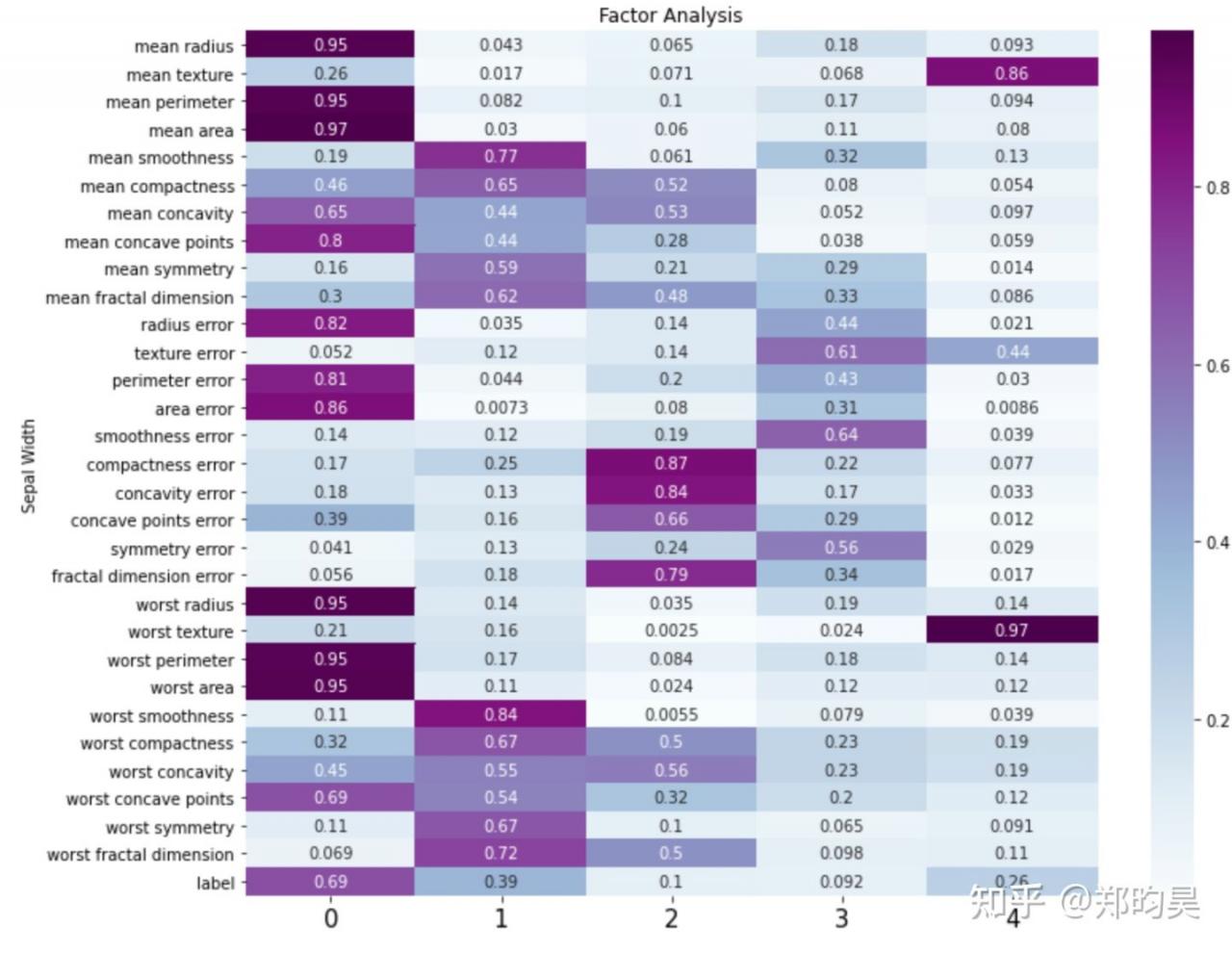

将原始数据转换为因子分析后的数据(5个隐藏因子)。
4 转换变量
pd.DataFrame(fa.transform(df))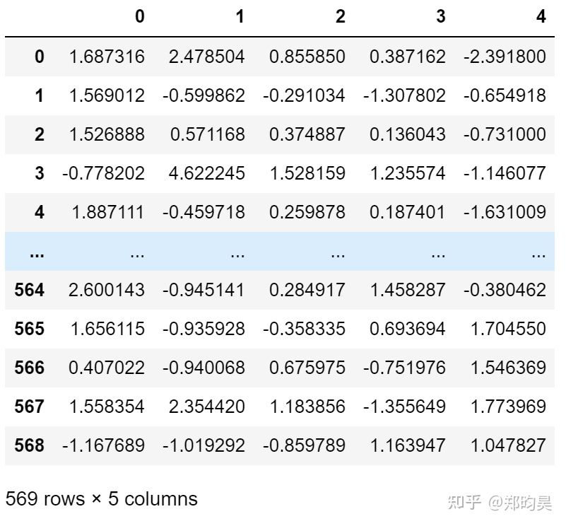

5 总结
因子分析在找到潜在隐藏变量的同时对数据进行了降维,是继PCA、LDA之后的又一大降维技术,有广泛的应用场景。
参考资料:
[1] https://mathpretty.com/10994.html
[2] 因子分析_百度百科
[3] 如何通俗地解释因子分析?
本文来自zhihu,观点不代表一起大数据-技术文章心得立场,如若转载,请注明出处:https://zhuanlan.zhihu.com/p/360848904
注意:本文归作者所有,未经作者允许,不得转载