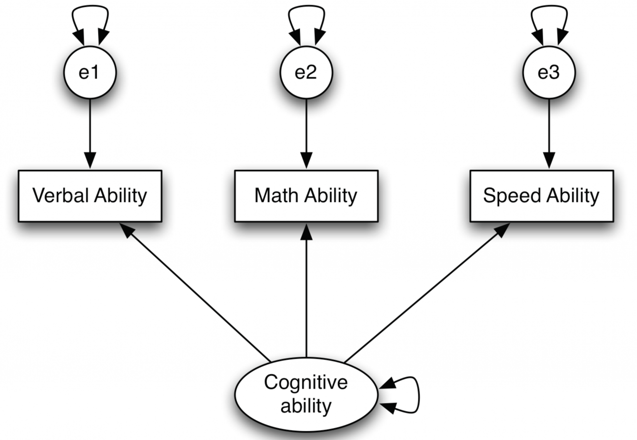

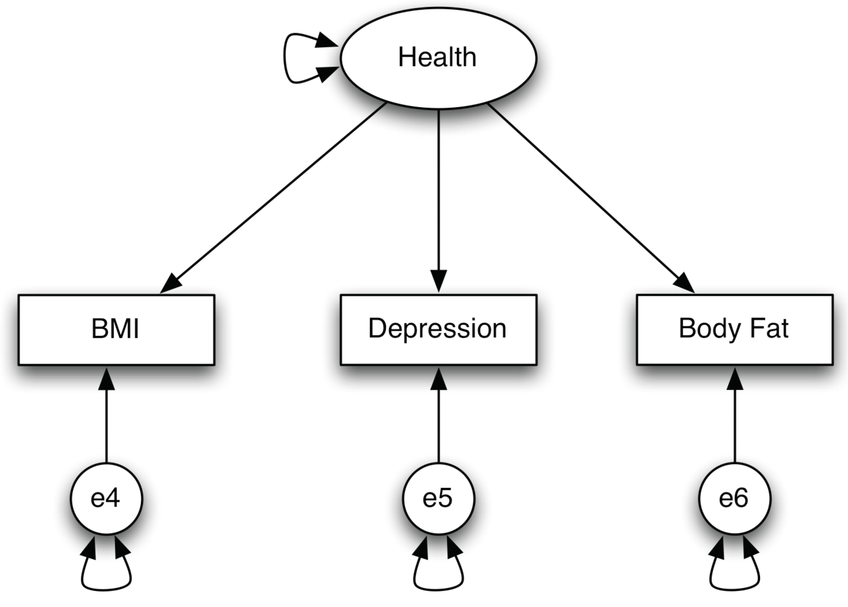
Figure 2 gives another example of measurement model – a model to measure health.

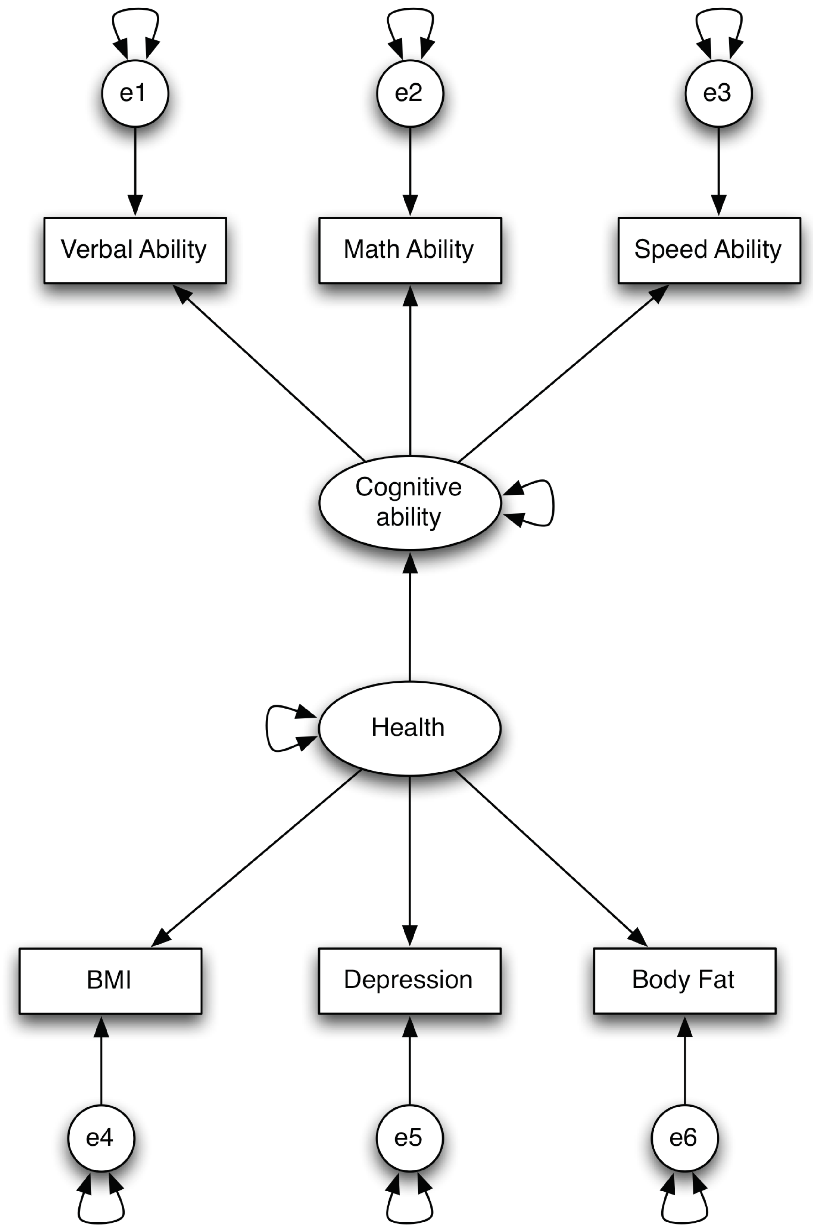
If one believes that health influences cognitive ability, then one can fit a path model using the factors – cognitive ability and health. Therefore, a structural model is actually a path model. Putting them together, we have a model in Figure 3. This model is called SEM model.

Example 1. Autoregressive model
In ACTIVE study, we have three variables – word series (ws), letter series (ls), and letter sets (ls) to measure reasoning ability. Also, we have data on all these three variables before and after training. Assume we want to test whether reasoning ability before training can predict reasoning ability after training. Then the SEM model in Figure 4 can be used. Not that we allow the factor in time 1 to predict the factor at time 2. In addition, we allow the uniqueness factors for each observed variable to be correlated. The R code for the analysis is given below.


First look at model fit. The chi-square value is 27 with 5 degrees of freedom. The p-value for chi-square test is almost 0. Thus, based on chi-square test, this is not a good model. However, CFI and TFI are both close to 1. The RMSEA is about 0.063 and SRMR is about 0.011. Considering the sample size here is large – N=1114, overall, we may accept this model is a fairly good model. Then we can answer our question. Because the regression coefficient from reasoning1 to reasoning2 is significant, reasoning ability before training seems to predict reasoning ability after training. In other words, those with higher reasoning ability before training tend to have higher reasoning ability after training.
> library(lavaan)
This is lavaan 0.5-23.1097
lavaan is BETA software! Please report any bugs.
> usedata('active.full.csv')
> automodel <- '
+ reasoning1 =~ ws1 + ls1 + lt1
+ reasoning2 =~ ws2 + ls2 + lt2
+ reasoning2 ~ reasoning1
+ ws1 ~~ ws2
+ ls1 ~~ ls2
+ lt1 ~~ lt2
+ '
>
> auto.res <- sem(automodel, data=active.full)
> summary(auto.res, fit=TRUE)
lavaan (0.5-23.1097) converged normally after  66 iterations

  Number of observations                          1114

  Estimator                                         ML
  Minimum Function Test Statistic               27.213
  Degrees of freedom                                 5
  P-value (Chi-square)                           0.000

Model test baseline model:

  Minimum Function Test Statistic             5827.630
  Degrees of freedom                                15
  P-value                                        0.000

User model versus baseline model:

  Comparative Fit Index (CFI)                    0.996
  Tucker-Lewis Index (TLI)                       0.989

Loglikelihood and Information Criteria:

  Loglikelihood user model (H0)             -16447.377
  Loglikelihood unrestricted model (H1)     -16433.771

  Number of free parameters                         16
  Akaike (AIC)                               32926.755
  Bayesian (BIC)                             33007.006
  Sample-size adjusted Bayesian (BIC)        32956.186

Root Mean Square Error of Approximation:

  RMSEA                                          0.063
  90 Percent Confidence Interval          0.041  0.087
  P-value RMSEA <= 0.05                          0.151

Standardized Root Mean Square Residual:

  SRMR                                           0.013

Parameter Estimates:

  Information                                 Expected
  Standard Errors                             Standard

Latent Variables:
                   Estimate  Std.Err  z-value  P(>|z|)
  reasoning1 =~
    ws1               1.000
    ls1               1.192    0.030   40.091    0.000
    lt1               0.422    0.016   26.301    0.000
  reasoning2 =~
    ws2               1.000
    ls2               1.110    0.026   43.371    0.000
    lt2               0.411    0.014   29.443    0.000

Regressions:
                   Estimate  Std.Err  z-value  P(>|z|)
  reasoning2 ~
    reasoning1        1.073    0.024   43.919    0.000

Covariances:
                   Estimate  Std.Err  z-value  P(>|z|)
 .ws1 ~~
   .ws2               1.216    0.327    3.718    0.000
 .ls1 ~~
   .ls2               0.356    0.401    0.888    0.375
 .lt1 ~~
   .lt2               1.596    0.138   11.544    0.000

Variances:
                   Estimate  Std.Err  z-value  P(>|z|)
   .ws1               5.511    0.385   14.324    0.000
   .ls1               4.547    0.475    9.575    0.000
   .lt1               3.996    0.181   22.065    0.000
   .ws2               5.021    0.419   11.995    0.000
   .ls2               5.161    0.507   10.182    0.000
   .lt2               3.963    0.181   21.875    0.000
    reasoning1       19.103    1.060   18.014    0.000
   .reasoning2        2.447    0.289    8.479    0.000

>
Example 2. Mediation analysis with latent variables
In path analysis, we have fitted a complex mediation model. Since we know that ws1, ls1, and lt1 are measurements of reasoning ability, we can form a latent reasoning ability variable. Thus, our mediation model can be expressed as in Figure 5.


Given CFI = 0.997, RMSEA = 0.034 and SRMR = 0.015, we accept the model as a good model even though the chi-square test is significant. Based on the Sobel test, the total indirect effect from age to ept1 through hvltt1 and reasoning is significant.
> library(lavaan)
This is lavaan 0.5-23.1097
lavaan is BETA software! Please report any bugs.
> usedata('active.full.csv')
> #head(active.full)
> med.model <- '
+ reasoning =~ ws1 + ls1 + lt1
+ reasoning ~ p4*age + p8*edu
+ hvltt1 ~ p2*age + p7*edu
+ hvltt1 ~~ reasoning
+ ept1 ~ p1*age + p6*edu + p3*hvltt1 + p5*reasoning
+ indirect := p2*p3 + p4*p5
+ total := p1 + p2*p3 + p7*p3
+ '
>
> med.res <- sem(med.model, data=active.full)
> summary(med.res, fit=TRUE)
lavaan (0.5-23.1097) converged normally after  51 iterations

  Number of observations                          1114

  Estimator                                         ML
  Minimum Function Test Statistic               18.363
  Degrees of freedom                                 8
  P-value (Chi-square)                           0.019

Model test baseline model:

  Minimum Function Test Statistic             3344.605
  Degrees of freedom                                20
  P-value                                        0.000

User model versus baseline model:

  Comparative Fit Index (CFI)                    0.997
  Tucker-Lewis Index (TLI)                       0.992

Loglikelihood and Information Criteria:

  Loglikelihood user model (H0)             -20675.968
  Loglikelihood unrestricted model (H1)     -20666.787

  Number of free parameters                         17
  Akaike (AIC)                               41385.937
  Bayesian (BIC)                             41471.204
  Sample-size adjusted Bayesian (BIC)        41417.207

Root Mean Square Error of Approximation:

  RMSEA                                          0.034
  90 Percent Confidence Interval          0.013  0.055
  P-value RMSEA <= 0.05                          0.889

Standardized Root Mean Square Residual:

  SRMR                                           0.015

Parameter Estimates:

  Information                                 Expected
  Standard Errors                             Standard

Latent Variables:
                   Estimate  Std.Err  z-value  P(>|z|)
  reasoning =~
    ws1               1.000
    ls1               1.181    0.029   41.262    0.000
    lt1               0.430    0.016   26.758    0.000

Regressions:
                   Estimate  Std.Err  z-value  P(>|z|)
  reasoning ~
    age       (p4)   -0.228    0.023   -9.737    0.000
    edu       (p8)    0.745    0.047   15.792    0.000
  hvltt1 ~
    age       (p2)   -0.161    0.027   -6.074    0.000
    edu       (p7)    0.429    0.052    8.177    0.000
  ept1 ~
    age       (p1)    0.030    0.022    1.389    0.165
    edu       (p6)    0.396    0.046    8.527    0.000
    hvltt1    (p3)    0.169    0.026    6.488    0.000
    reasoning (p5)    0.643    0.035   18.186    0.000

Covariances:
                   Estimate  Std.Err  z-value  P(>|z|)
 .reasoning ~~
   .hvltt1            7.255    0.592   12.263    0.000

Variances:
                   Estimate  Std.Err  z-value  P(>|z|)
   .ws1               5.334    0.366   14.594    0.000
   .ls1               4.850    0.444   10.910    0.000
   .lt1               3.917    0.181   21.657    0.000
   .hvltt1           20.618    0.874   23.601    0.000
   .ept1             11.505    0.522   22.027    0.000
   .reasoning        13.814    0.777   17.777    0.000

Defined Parameters:
                   Estimate  Std.Err  z-value  P(>|z|)
    indirect         -0.174    0.019   -9.368    0.000
    total             0.075    0.025    3.008    0.003

>
本文来自advstats.psychstat.org,观点不代表一起大数据-技术文章心得立场,如若转载,请注明出处:https://advstats.psychstat.org/book/sem/index.php
注意:本文归作者所有,未经作者允许,不得转载