本次用到的数据是kaggle北京链家网2002年到2018年的二手房买卖成交数据,地址如下:
https://www.kaggle.com/c/house-prices-advanced-regression-techniques
本文是为了对链家,安居客等平台二手房估价系统采用的估价模型进行探索,主要是为了在实际应用,而不是参与比赛,模型或者很多方面没有使用很高深的研究。
1 分析目的
基于Kaggle提供的北京链家网2002年到2018年的二手房买卖成交数据,探索链家二手房估价系统。
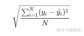
模型的评估指标是,用于回归问题的常见指标——均方根误差 (RMSE):
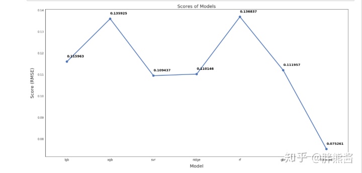
从上图中可以看出,混合模型的RMSLE为0.075,远远优于其他模型。这是本次用来做最终预测的模型。
2 数据收集
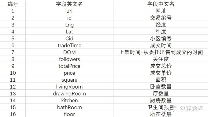
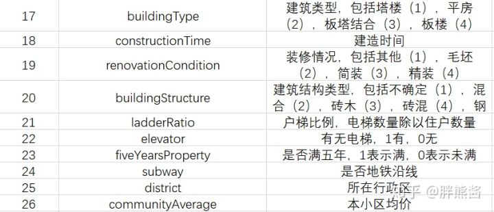
Kaggle提供的数据共计,26个字段,318852行。
数据详细描述:
3 数据清洗
3.1 选择子集
网址,经度,维度,id,Cid跟本次房价预测模型无关,可以选择删除。
3.2 删除重复值
Excel删除26条重复值。
3.3 数据一致化
未知全改为nan。
drawingRoom和floor明显有错位替换。
floor这里,为了方便后续建模,把floor分列floorType,floorNum,高-H-1,中-M-2,低-L-3,底-D-4,顶-U-5,钢混结构和混合结构和楼层无关,全改为nan。floor改为数值格式。
以防后续建模不方便,全部改为数值格式。
3.4 删除异常值
时间和价格的关系
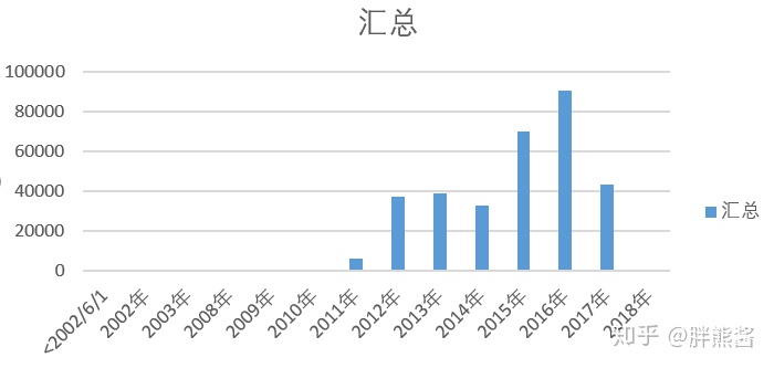
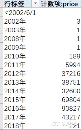
2010以前的数据很少,基本不对价格造成什么影响,予以删除。
3.5 导入数据
#必须导入的包
import pandas as pd
import numpy as np

# 图形
import matplotlib.pyplot as plt
import seaborn as sns

# 统计
from scipy import stats
from scipy.stats import skew, norm
from subprocess import check_output
from scipy.special import boxcox1p
from scipy.stats import boxcox_normmax

# 分类
from sklearn.model_selection import GridSearchCV
from sklearn.model_selection import KFold, cross_val_score
from sklearn.metrics import mean_squared_error
from sklearn.preprocessing import OneHotEncoder
from sklearn.preprocessing import LabelEncoder
from sklearn.pipeline import make_pipeline
from sklearn.preprocessing import scale
from sklearn.preprocessing import StandardScaler
from sklearn.preprocessing import RobustScaler
from sklearn.decomposition import PCA

# 模型
from sklearn.ensemble import RandomForestRegressor, GradientBoostingRegressor, AdaBoostRegressor, BaggingRegressor
from sklearn.kernel_ridge import KernelRidge
from sklearn.pipeline import make_pipeline
from sklearn.preprocessing import RobustScaler
from sklearn.linear_model import Ridge, RidgeCV
from sklearn.linear_model import ElasticNet, Lasso,  BayesianRidge, LassoLarsIC
from sklearn.svm import SVR
from mlxtend.regressor import StackingCVRegressor
import lightgbm as lgb
from lightgbm import LGBMRegressor
from sklearn.base import BaseEstimator, TransformerMixin, RegressorMixin, clone
from sklearn.model_selection import KFold, cross_val_score, train_test_split
from sklearn.metrics import mean_squared_error
import xgboost as xgb
from xgboost import XGBRegressor

#导入数据集
erhouse = pd.read_csv('Lianjiaerhouse.csv',encoding='gbk')

#数据集指标检查
erhouse.columns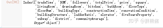
3.6 数据观察
我们的目标是根据这些特征预测销售价格。
围绕价格展开特征的研究
样本和特征的数量
print('The data size is : {} '.format(erhouse.shape))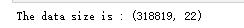

数据的前五列
erhouse.head(5)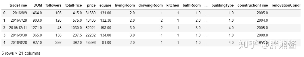
price销售价格是需要预测的变量。
price的分布
sns.distplot(erhouse['price'])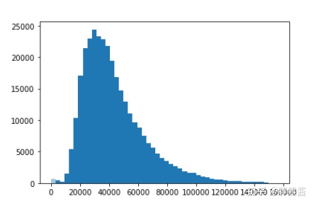
集中在20000-50000价格区间。
偏度和峰值
#skewness and kurtosis
print('Skewness: %f' % erhouse['price'].skew())
print('Kurtosis: %f' % erhouse['price'].kurt())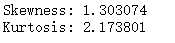
偏度为 1.303074和峰值2.173801。
3.7 异常值处理
异常值是在数据集中不合理存在的值,也称为离群点,是样本数据的干扰数据。
前面我们已经处理过时间特征的异常值,接下来,我们会对其它特征进行探索,尽可能减少干扰数据。
我们可以通过描述性统计或正态分布等统计方法查看异常值,具体的异常值划分标准以个人经验和实际情况决定。
异常值处理方法:删除(最简单粗暴的方法,会对整体数据分布造成不良影响);按照缺失值处理方法进行;用均值,中位数等数据填充(本文采用的方法);不处理。
本文主要探索各特征与价格预测之间的关系,异常值也围绕它们之间的关系展开。
先用热力图并绘制出这些特征之间,以及它们与销售价格之间的关系。
所有特征热力图
corrmat = erhouse.corr()
f, ax = plt.subplots(figsize=(12, 9))
sns.heatmap(corrmat, vmax=.8, square=True);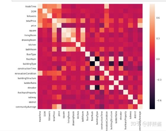
可以很直观的看到特征与特征之间以及特征与价格之间的相关性强弱。
没有tradeTime为什么?
从上图可以看出,20个特征和价格的相关性有强有弱,那么,为了更好的剔除异常值,我们按照上图的强弱顺序,五个一组的对特征和价格的联系进行进一步的研究,最终发现异常值。
price和特征1-5的散点图
sns.set()
cols = [ 'tradeTime', 'DOM', 'followers', 'totalPrice', 'square', 'price']
sns.pairplot(erhouse[cols], size = 2.5)
plt.show();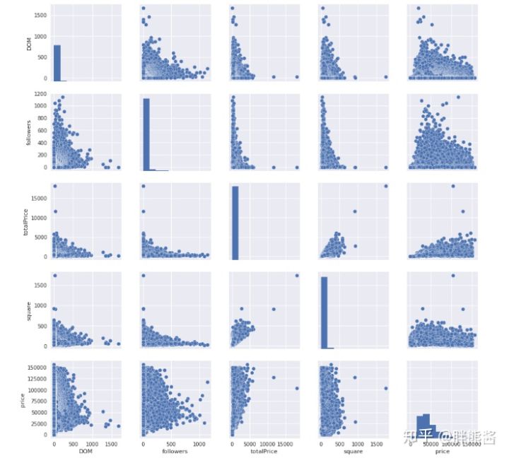
tradeTime又没有出现,不管了。
从上面这些图中,我们能够很直观的看到这些特征以及它们与价格之间的联系都比较紧密,但是以上四个特征都有明显的异常值。
接下来,我们对这这些特征和SalePrice的进行进一步的探索。
price和DOM
var = 'DOM'
data = pd.concat([erhouse['price'], erhouse[var]], axis=1)
data.plot.scatter(x=var, y='price', ylim=(0,150000));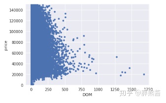
上图透露当DOM更大时,看起来相关性更弱,并且远离点群。
最右边的几个点,离数据点群非常的远,且不符合整体的图表走势,显然是异常值,但是,删除太多可能最后造成过拟合的结果,我们可以选择删除就删除最右边的值。
erhouse.sort_values(by = 'DOM', ascending = False)[:2]
erhouse = erhouse.drop(erhouse[erhouse['DOM'] == 1677].index)
删除以后再看
var = 'DOM'
data = pd.concat([erhouse['price'], erhouse[var]], axis=1)
data.plot.scatter(x=var, y='price', ylim=(0,150000));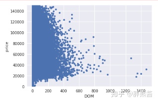
price和followers
var = 'followers'
data = pd.concat([erhouse['price'], erhouse[var]], axis=1)
data.plot.scatter(x=var, y='price', ylim=(0,150000));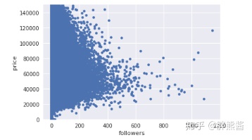
上图异常情况不是很显著,不予删除。
price和totalPrice
var = 'totalPrice'
data = pd.concat([erhouse['price'], erhouse[var]], axis=1)
data.plot.scatter(x=var, y='price', ylim=(0,150000));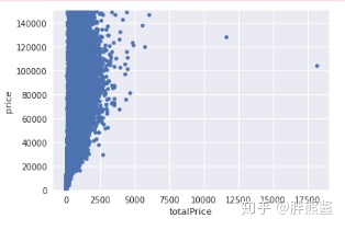
依旧选择只删除最右边,最显著的那个点。
erhouse.sort_values(by = 'totalPrice', ascending = False)[:2]
erhouse = erhouse.drop(erhouse[erhouse['totalPrice'] == 18130].index)
删除后
var = 'totalPrice'
data = pd.concat([erhouse['price'], erhouse[var]], axis=1)
data.plot.scatter(x=var, y='price', ylim=(0,150000));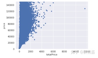
price和square
var = 'square'
data = pd.concat([erhouse['price'], erhouse[var]], axis=1)
data.plot.scatter(x=var, y='price', ylim=(0,150000));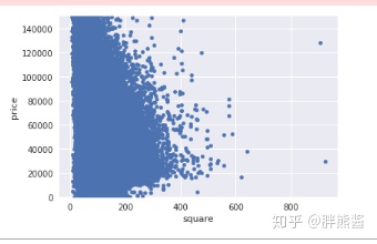
依旧选择只删除最右边,最显著的2个点。
erhouse.sort_values(by = 'square', ascending = False)[:2]
erhouse = erhouse.drop(erhouse[erhouse['square'] == 906].index)
erhouse = erhouse.drop(erhouse[erhouse['square'] ==922.7].index)
删除后
var = 'square'
data = pd.concat([erhouse['price'], erhouse[var]], axis=1)
data.plot.scatter(x=var, y='price', ylim=(0,150000));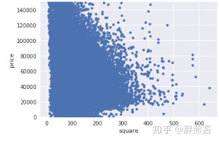
price和特征6-11的散点图
sns.set()
cols = [ 'livingRoom', 'drawingRoom', 'kitchen', 'bathRoom', 'floorType', 'floorNum', 'price']
sns.pairplot(erhouse[cols], size = 2.5)
plt.show();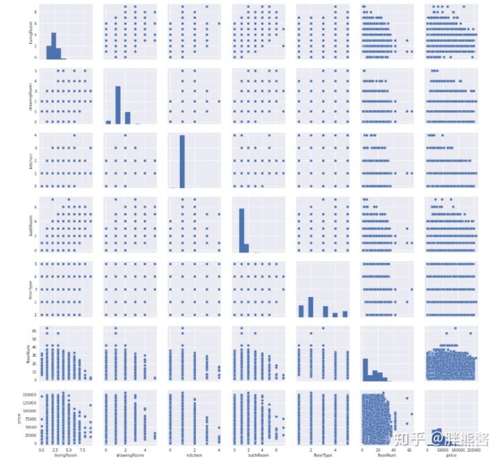
没有很明显的趋势,也看不出明显的异常情况。
但是,竟然被我发现bathRoom和constructionTime貌似错位了,换回来,代码重新run一遍。
price和特征12-16的散点图
sns.set()
cols = [ 'buildingType', 'constructionTime', 'renovationCondition', 'buildingStructure', 'ladderRatio', 'price']
sns.pairplot(erhouse[cols], size = 2.5)
plt.show();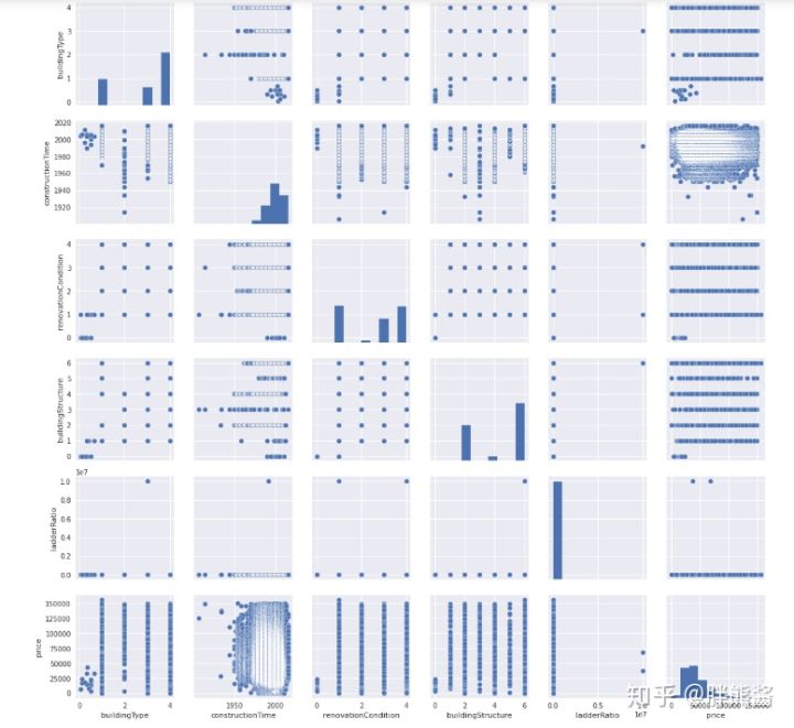
ladderRatio异常情况较为明显。
price和ladderRatio
var = 'ladderRatio'
data = pd.concat([erhouse['price'], erhouse[var]], axis=1)
data.plot.scatter(x=var, y='price', ylim=(0,150000));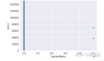
依旧选择只删除最右边,最显著的2个点。
erhouse.sort_values(by = 'ladderRatio', ascending = False)[:2]
erhouse = erhouse.drop(erhouse[erhouse['ladderRatio'] ==10009400].index)
删除后
var = 'ladderRatio'
data = pd.concat([erhouse['price'], erhouse[var]], axis=1)
data.plot.scatter(x=var, y='price', ylim=(0,150000));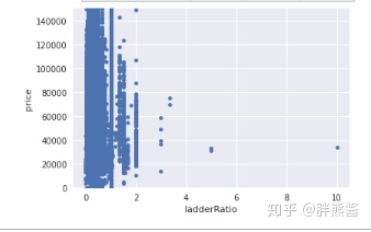
勉强可以,剩下的就不处理了。
price和特征17-21的散点图
sns.set()
cols = [ 'elevator', 'fiveYearsProperty', 'subway', 'district', 'communityAverage', 'price']
sns.pairplot(erhouse[cols], size = 2.5)
plt.show();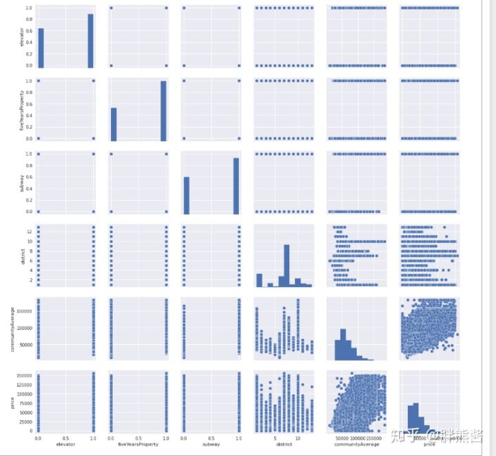
看不太出来明显的异常,不处理。
删除后还剩多少数据
erhouse.shape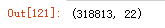

3.8 目标变量处理
下面我们将通过直方图来看SalePrice的分布:
sns.distplot(erhouse['price'], fit=norm);
fig = plt.figure()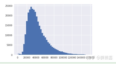
可以看出,销售价格在右边倾斜,是非正态分布数据。因为大多数机器学习模型不能很好地处理非正态分布数据,应用log(1+x)变换来修正倾斜。
erhouse['price'] = np.log(erhouse['price'])再画一次销售价格的分布:
sns.distplot(erhouse['price'], fit=norm);
fig = plt.figure()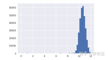
分离特征和标签
erhouse_labels = erhouse['price'].reset_index(drop=True)
features = erhouse.drop(['price'], axis=1)
特征数量
features.shape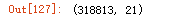

3.9 缺失值处理
缺失值会对样本量产生影响,进而影响到整体数据质量。所以,我们应该对缺失值进行更多的探索,以使我们的数据完整,更能符合建模的需要。
缺失值探索
features_na = (features.isnull().sum() / len(features)) * 100
features_na = features_na.drop(features_na[features_na == 0].index).sort_values(ascending=False)[:30]
missing_data = pd.DataFrame({'Missing Ratio' :features_na})
missing_data.head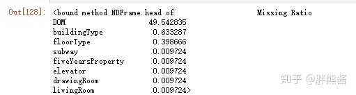
特征缺失较为明显,需要集中进行处理。
几种常见的缺失值处理方法:
删除:删除缺失特征或者单条数据。但是,会造成大量数据的浪费,同时造成样本整体的不均匀。
缺失值插补:人工填写;特殊值填充;替换填充(用未缺失的数据的均值填充,众数填充,中位数填充,拉格朗日插值填充);预测填充。(本文主要采用的是插补的方法。)
缺失值插补
#用平均值替换掉缺失值。
#DOM为上架时间,可以用平均时间28.82319154替换
features['DOM'] = features['DOM'] .fillna(28.82319154)
#buildingType为建筑类型,可以用常见的4(板楼)替换
features['buildingType'] = features['buildingType'] .fillna(4)
#floorType为所在楼层类型,可以用常见 2
features['floorType'] = features['floorType'] .fillna('2')
#drawingRoom为厅数量,可以用平均时间1替换
features['drawingRoom'] = features['drawingRoom'] .fillna(1)

#用0替换掉缺失值。
#livingRoom代表没有卧室,很迷啊,但是也不能随意增加,还是用0代替吧
features['livingRoom'] = features['livingRoom'].fillna(0)
#elevator,fiveYearsProperty,subway分别代表没有电梯,没有满五年,没有地铁,用0代替。
for col in ('elevator', 'fiveYearsProperty', 'subway'):
    features[col] = features[col].fillna(0)


#在原始数据改
#constructionTime有19283nan,返回去修改原始数据,按照tradetime减去DOM时间估算。
#communityAverage为区域均价,这个还涉及到一个不同年份价格的影响不同的问题,这里,我采取,按当年份区域均价补充的方法,
#介于代码不好写,继续在原始数据改,改为重新run
#缺失值删除
是否还有缺失?
是否还有缺失?
features_na = (features.isnull().sum() / len(features)) * 100
features_na = features_na.drop(features_na[features_na == 0].index).sort_values(ascending=False)[:30]
missing_data = pd.DataFrame({'Missing Ratio' :features_na})
missing_data.head
没有缺失值。
4 特征工程
“数据决定了机器学习的上限,而算法只是尽可能逼近这个上限”,这里的数据指的就是经过特征工程得到的数据。特征工程指的是把原始数据通过特征构建、特征处理等操作转变为模型的训练数据的过程,它的目的就是获取更好的训练数据特征,使得机器学习模型逼近这个上限。特征工程能使得模型的性能得到提升,有时甚至在简单的模型上也能取得不错的效果。
4.1 数据转换
机器学习中,为了让杂乱的数据变得更规整,以满足数据分析或建模的需要。需要通过数据转换对数据进行规范化处理。这就是对特征进行处理,将原始数据转变为模型的训练数据。
数据的规范化处理有利于排除或者减弱数据异常的影响,从而可以提升模型效率。
数据转换的方式有很多种,比较常用的有对数转换,box-cox转换等变换方式。
在数据清洗-目标变量SalePrice环节, 采用了对数转换对数据进行规范化处理,这里,我们将采用box-cox转换。
数据转换是针对数据变量进行的特征处理,先找出数值特征。
找到数值特征
numeric_dtypes = ['int16', 'int32', 'int64', 'float16', 'float32', 'float64']
numeric = []
for i in features.columns:
    if features[i].dtype in numeric_dtypes:
        numeric.append(i)
找到倾斜的数值特征
skew_features = features[numeric].apply(lambda x: skew(x)).sort_values(ascending=False)

high_skew = skew_features[skew_features > 0.5]
skew_index = high_skew.index

print('There are {} numerical features with Skew > 0.5 :'.format(high_skew.shape[0]))
skewness = pd.DataFrame({'Skew' :high_skew})
skew_features.head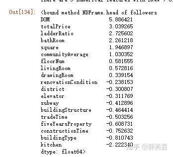
我们用scipy函数boxcox1p来计算Box-Cox转换。我们的目标是找到一个简单的转换方式使数据规范化。
倾斜特征正规化
for i in skew_index:
    features[i] = boxcox1p(features[i], boxcox_normmax(features[i] + 1))
确认是否处理完所有倾斜特征。
skew_features = features[numeric].apply(lambda x: skew(x)).sort_values(ascending=False)
high_skew = skew_features[skew_features > 0.5]
skew_index = high_skew.index
print('There are {} numerical features with Skew > 0.5 :'.format(high_skew.shape[0]))
skewness = pd.DataFrame({'Skew' :high_skew})
skew_features.head
现在,所有的特征看起来都是正态分布的了。
4.2 增加特征
增加特征主要是利用已有的特征进行一系列处理进行变量的延伸,可以是简单的特征加减乘除等。主要是凭借对数据的理解进行进一步的加工, 所以我们可以基于对数据集的理解创建一些特征来帮助我们的模型。(新特征的构建应该符合真实的业务逻辑,这样才能构建真正有价值的特征。)
#通过加总的特征
#卧室,厨房,卫生间等全部相加
features['TotalNum'] = features['livingRoom'] +features['kitchen']+features['bathRoom']
#建筑类型,装修情况,建筑结构类型,是否满五年,是否有电梯,是否地铁沿线等全部相加
features['TotalYN'] = (features['buildingType'] + features['renovationCondition'] +features['buildingStructure']
+features['fiveYearsProperty']+features['elevator']+features['subway'])

#通过相乘的特征
#市场价=区域价格*面积
features['TotaMprice'] = features['communityAverage'] * features['square']
4.3 特征转换
我们通过计算数值特征的对数和平方变换来创建更多的特征。
#通过对数处理获得新的特征
def logs(res, ls):
    m = res.shape[1]
    for l in ls:
        res = res.assign(newcol=pd.Series(np.log(1.01+res[l])).values)
        res.columns.values[m] = l + '_log'
        m += 1
    return res

log_features = ['DOM','followers','totalPrice','square','livingRoom','kitchen',
                 'bathRoom','buildingType','renovationCondition','buildingStructure','ladderRatio',
                 'district','communityAverage']

features = logs(features, log_features)

log_features =  ['DOM','followers','totalPrice','square','livingRoom','kitchen',
                 'bathRoom','buildingType','renovationCondition','buildingStructure','ladderRatio',
                 'district','communityAverage']


features = logs(features, log_features)
#通过平方转换获得新的特征
def squares(res, ls):
    m = res.shape[1]
    for l in ls:
        res = res.assign(newcol=pd.Series(res[l]*res[l]).values)
        res.columns.values[m] = l + '_sq'
        m += 1
    return res

squared_features = ['DOM','followers','totalPrice','square','livingRoom','kitchen',
                 'bathRoom','buildingType','renovationCondition','buildingStructure','ladderRatio',
                 'district','communityAverage']

features = squares(features, squared_features)
查看特征数
features.shape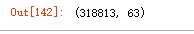
新增43个特征。
4.4 字符型特征的独热编码
查看当前的数据情况:
features.info()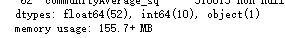
floorType为文本,转换成数值
features['floorType'] = features['floorType'].astype(int)再看:
features.info()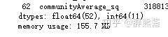
至此,所有字符型特征变量都成了数值型特征。
4.5 特征降维
在前面的特征转换,新增等操作中,我们新增了43个特征,现在一共有63个特征,特征量较少,为了避免降纬,遗失重要信息,不予以降纬。
5 数据建模
建模也就是根据所研究的问题选择恰当的算法搭建学习模型,并且基于所设定的模型评价指标,在训练过程中调整模型参数以使得模型的整体性能达到最优。
在Kaggle的比赛中优胜方案通常都会做模型集成(ensemble),模型集成会整合不同模型的预测结果,生成最终预测,集成的模型越多,效果就越好。
这里介于我们是工作中使用,没有采用比赛中高端集成方案,只做简单的结果加权。
5.1.1 数据准备
查看集
erhouse_labels.shape, features.shape5.1.2 主成分分析(PCA)
前面新增的这些特征都是和原始特征高度相关的,但这可能导致较强的多重共线性 (Multicollinearity) 。可以利用PCA去除相关性,提升模型训练的效果。
PCA的思想是通过坐标轴转换,寻找数据分布的最优子空间,从而达到降维、去相关的目的。
因为这里使用PCA的目的不是降维,所以 n_components 用了和原来差不多的维度,即前面加XX特征,后面再降到XX维。
pca_model = PCA(n_components=63)
Features= pca_model.fit_transform(features)
5.2 设置交叉验证并定义错误度量
在前面我们已经获得训练集用作训练模型,而在训练模型环节,为了防止模型过拟合,我们又对训练集进行交叉验证。
这里我简单粗暴的应用K折交叉验证法,每次的训练集将不再只包含一组数据,而是多组,具体数目将根据K的选取决定。比如,如果K=5,那么我们利用五折交叉验证的步骤就是:
1)将训练集分成5份
2)不重复地每次取其中一份做测试,用其他四份做训练,之后计算该模型在测试集上的rmse
3)将5次的rmse平均得到最后的rmse
# 设置交叉验证
kf = KFold(n_splits=5, random_state=42, shuffle=True)

# 定义错误度量
def rmsle(y, y_pred):
    return np.sqrt(mean_squared_error(y, y_pred))

def cv_rmse(model, X=Features):
    rmse = np.sqrt(-cross_val_score(model, X, erhouse_labels, scoring="neg_mean_squared_error", cv=kf))
    return (rmse)
5.3 设置模型
这次直接选用常用的lightgbm,XGBoost, RandomForestRegressor模型。
lightgbm = LGBMRegressor(objective='regression',
                       num_leaves=6,
                       learning_rate=0.01,
                       n_estimators=7000,
                       max_bin=200,
                       bagging_fraction=0.8,
                       bagging_freq=4,
                       bagging_seed=8,
                       feature_fraction=0.2,
                       feature_fraction_seed=8,
                       min_sum_hessian_in_leaf = 11,
                       verbose=-1,
                       random_state=42)

xgboost = XGBRegressor(learning_rate=0.01,
                       n_estimators=6000,
                       max_depth=4,
                       min_child_weight=0,
                       gamma=0.6,
                       subsample=0.7,
                       colsample_bytree=0.7,
                       objective='reg:linear',
                       nthread=-1,
                       scale_pos_weight=1,
                       seed=27,
                       reg_alpha=0.00006,
                       random_state=42)

rf = RandomForestRegressor(n_estimators=1200,
                          max_depth=15,
                          min_samples_split=5,
                          min_samples_leaf=5,
                          max_features=None,
                          oob_score=True,
                          random_state=42)
5.4 模型得分
获得每个模型的交叉验证分数。
scores = {}

score = cv_rmse(lightgbm)
print('lightgbm: {:.4f} ({:.4f})'.format(score.mean(), score.std()))
scores['lgb'] = (score.mean(), score.std())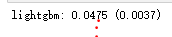
score = cv_rmse(xgboost)
print('xgboost: {:.4f} ({:.4f})'.format(score.mean(), score.std()))
scores['xgb'] = (score.mean(), score.std())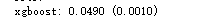

score = cv_rmse(rf)
print('rf: {:.4f} ({:.4f})'.format(score.mean(), score.std()))
scores['rf'] = (score.mean(), score.std())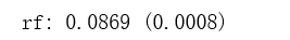
5.5 安装模型
print('lightgbm')
lgb_model_full_data = lightgbm.fit(Features,erhouse_labels)

print('xgboost')
xgb_model_full_data = xgboost.fit(Features,erhouse_labels)

print('RandomForest')
rf_model_full_data = rf.fit(Features,erhouse_labels)

5.6 加权模型结果得到预测值
def sumed_predictions(Features):
return ((0.3 * xgb_model_full_data.predict(Features)) +
            (0.4 * lgb_model_full_data.predict(Features)) +
            (0.3 * rf_model_full_data.predict(Features))))
得到加权模型的预测得分,不断修改参数,得到最优模型权重。
sumed_score = rmsle(erhouse_labels, sumed_predictions(Features))
scores['sumed'] = (sumed_score, 0)
print('RMSLE score on data:')
print(sumed_score)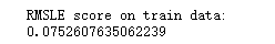
5.7 确定性能最佳的模型
图形展示所有模型的预测结果。
sns.set_style("white")
fig = plt.figure(figsize=(24, 12))

ax = sns.pointplot(x=list(scores.keys()), y=[score for score, _ in scores.values()], markers=['o'], linestyles=['-'])
for i, score in enumerate(scores.values()):
    ax.text(i, score[0] + 0.002, '{:.6f}'.format(score[0]), horizontalalignment='left', size='large', color='black', weight='semibold')

plt.ylabel('Score (RMSE)', size=20, labelpad=12.5)
plt.xlabel('Model', size=20, labelpad=12.5)
plt.tick_params(axis='x', labelsize=13.5)
plt.tick_params(axis='y', labelsize=12.5)

plt.title('Scores of Models', size=20)

plt.show()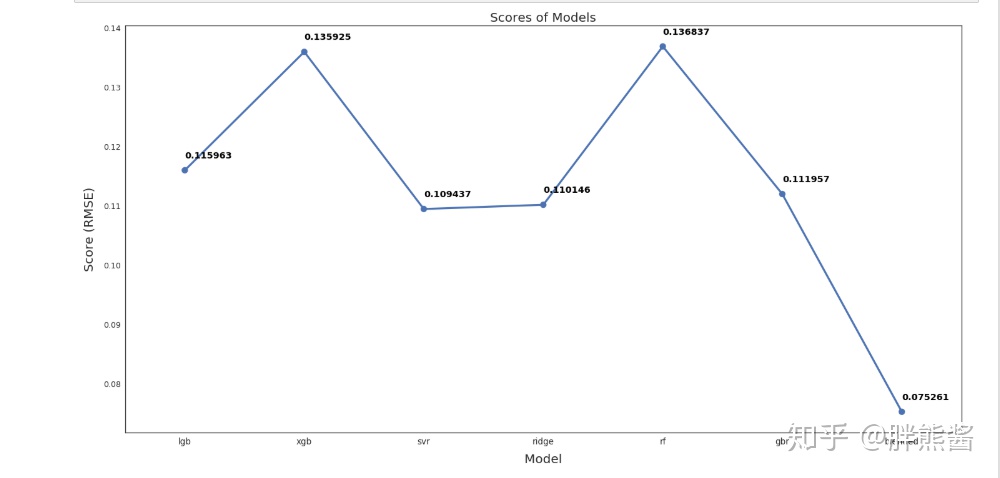
从上图中我们可以看出,加权模型的RMSLE为0.075,远远优于其他模型。这是我用来做最终预测的模型。
6 封装模型
model = sumed_predictions(Features)#模型封装
from sklearn.externals import joblib
joblib.dump(model,'model.pkl')
ml= joblib.load('model.pkl')
7 调用模型
输入数据调用模型
本文来自知乎,观点不代表一起大数据-技术文章心得立场,如若转载,请注明出处:https://zhuanlan.zhihu.com/p/159085585
注意:本文归作者所有,未经作者允许,不得转载