from http://machinelearningmastery.com/machine-learning-in-r-step-by-step/
Do you want to do machine learning using R, but you’re having trouble getting started?
In this post you will complete your first machine learning project using R.
In this step-by-step tutorial you will:
- Download and install R and get the most useful package for machine learning in R.
- Load a dataset and understand it’s structure using statistical summaries and data visualization.
- Create 5 machine learning models, pick the best and build confidence that the accuracy is reliable.
If you are a machine learning beginner and looking to finally get started using R, this tutorial was designed for you.
Let’s get started!
How Do You Start Machine Learning in R?
The best way to learn machine learning is by designing and completing small projects.
R Can Be Intimidating When Getting Started
R provides a scripting language with an odd syntax. There are also hundreds of packages and thousands of functions to choose from, providing multiple ways to do each task. It can feel overwhelming.
The best way to get started using R for machine learning is to complete a project.
- It will force you to install and start R (at the very least).
- It will given you a bird’s eye view of how to step through a small project.
- It will give you confidence, maybe to go on to your own small projects.
Beginners Need A Small End-to-End Project
Books and courses are frustrating. They give you lots of recipes and snippets, but you never get to see how they all fit together.
When you are applying machine learning to your own datasets, you are working on a project.
A machine learning project may not be linear, but it has a has a number of well known steps:
- Define Problem.
- Prepare Data.
- Evaluate Algorithms.
- Improve Results.
- Present Results.
For more information on the steps in a machine learning project see this checklist and more on the process.
The best way to really come to terms with a new platform or tool is to work through a machine learning project end-to-end and cover the key steps. Namely, from loading data, summarizing your data, evaluating algorithms and making some predictions.
If you can do that, you have a template that you can use on dataset after dataset. You can fill in the gaps such as further data preparation and improving result tasks later, once you have more confidence.
Hello World of Machine Learning
The best small project to start with on a new tool is the classification of iris flowers (e.g. the iris dataset).
This is a good project because it is so well understood.
- Attributes are numeric so you have to figure out how to load and handle data.
- It is a classification problem, allowing you to practice with perhaps an easier type of supervised learning algorithms.
- It is a mutli-class classification problem (multi-nominal) that may require some specialized handling.
- It only has 4 attribute and 150 rows, meaning it is small and easily fits into memory (and a screen or A4 page).
- All of the numeric attributes are in the same units and the same scale not requiring any special scaling or transforms to get started.
Let’s get started with your hello world machine learning project in R.
Machine Learning in R: Step-By-Step Tutorial (start here)
In this section we are going to work through a small machine learning project end-to-end.
Here is an overview what we are going to cover:
- Installing the R platform.
- Loading the dataset.
- Summarizing the dataset.
- Visualizing the dataset.
- Evaluating some algorithms.
- Making some predictions.
Take your time. Work through each step.
Try to type in the commands yourself or copy-and-paste the commands to speed things up.
Any questions, please leave a comment at the bottom of the post.
1. Downloading Installing and Starting R
Get the R platform installed on your system if it is not already.
UPDATE: This tutorial was written and tested with R version 3.2.3. It is recommend that you use this version of R or higher.
I do not want to cover this in great detail, because others already have. This is already pretty straight forward, especially if you are a developer. If you do need help, ask a question in the comments.
Here is what we are going to cover in this step:
- Download R.
- Install R.
- Start R.
- Install R Packages.
1.1 Download R
You can download R from The R Project webpage.
When you click the download link, you will have to choose a mirror. You can then choose R for your operating system, such as Windows, OS X or Linux.
1.2 Install R
R is is easy to install and I’m sure you can handle it. There are no special requirements. If you have questions or need help installing see R Installation and Administration.
1.3 Start R
You can start R from whatever menu system you use on your operating system.
For me, I prefer the command line.
Open your command line, change (or create) to your project directory and start R by typing:
|
1
|
R
|
You should see something like the screenshot below either in a new window or in your terminal.
R Interactive Environment
1.4 Install Packages
Install the packages we are going to use today. Packages are third party add-ons or libraries that we can use in R.
|
1
|
install.packages(“caret”)
|
UPDATE: We may need other packages, but caret should ask us if we want to load them. If you are having problems with packages, you can install the caret packages and all packages that you might need by typing:
|
1
|
install.packages(“caret”, dependencies=c(“Depends”, “Suggests”))
|
Now, let’s load the package that we are going to use in this tutorial, the caret package.
|
1
|
library(caret)
|
The caret package provides a consistent interface into hundreds of machine learning algorithms and provides useful convenience methods for data visualization, data resampling, model tuning and model comparison, among other features. It’s a must have tool for machine learning projects in R.
For more information about the caret R package see the caret package homepage.
2. Load The Data
We are going to use the iris flowers dataset. This dataset is famous because it is used as the “hello world” dataset in machine learning and statistics by pretty much everyone.
The dataset contains 150 observations of iris flowers. There are four columns of measurements of the flowers in centimeters. The fifth column is the species of the flower observed. All observed flowers belong to one of three species.
You can learn more about this dataset on Wikipedia.
Here is what we are going to do in this step:
- Load the iris data the easy way.
- Load the iris data from CSV (optional, for purists).
- Separate the data into a training dataset and a validation dataset.
Choose your preferred way to load data or try both methods.
2.1 Load Data The Easy Way
Fortunately, the R platform provides the iris dataset for us. Load the dataset as follows:
|
1
2
3
4
|
# attach the iris dataset to the environment
data(iris)
# rename the dataset
dataset <– iris
|
You now have the iris data loaded in R and accessible via the dataset variable.
I like to name the loaded data “dataset”. This is helpful if you want to copy-paste code between projects and the dataset always has the same name.
2.2 Load From CSV
Maybe your a purist and you want to load the data just like you would on your own machine learning project, from a CSV file.
- Download the iris dataset from the UCI Machine Learning Repository (here is the direct link).
- Save the file as iris.csv your project directory.
Load the dataset from the CSV file as follows:
|
1
2
3
4
5
6
|
# define the filename
filename <– “iris.csv”
# load the CSV file from the local directory
dataset <– read.csv(filename, header=FALSE)
# set the column names in the dataset
colnames(dataset) <– c(“Sepal.Length”,“Sepal.Width”,“Petal.Length”,“Petal.Width”,“Species”)
|
You now have the iris data loaded in R and accessible via the dataset variable.
2.3. Create a Validation Dataset
We need to know that the model we created is any good.
Later, we will use statistical methods to estimate the accuracy of the models that we create on unseen data. We also want a more concrete estimate of the accuracy of the best model on unseen data by evaluating it on actual unseen data.
That is, we are going to hold back some data that the algorithms will not get to see and we will use this data to get a second and independent idea of how accurate the best model might actually be.
We will split the loaded dataset into two, 80% of which we will use to train our models and 20% that we will hold back as a validation dataset.
|
1
2
3
4
5
6
|
# create a list of 80% of the rows in the original dataset we can use for training
validation_index <– createDataPartition(dataset$Species, p=0.80, list=FALSE)
# select 20% of the data for validation
validation <– dataset[–validation_index,]
# use the remaining 80% of data to training and testing the models
dataset <– dataset[validation_index,]
|
You now have training data in the dataset variable and a validation set we will use later in thevalidation variable.
Note that we replaced our dataset variable with the 80% sample of the dataset. This was an attempt to keep the rest of the code simpler and readable.
3. Summarize Dataset
Now it is time to take a look at the data.
In this step we are going to take a look at the data a few different ways:
- Dimensions of the dataset.
- Types of the attributes.
- Peek at the data itself.
- Levels of the class attribute.
- Breakdown of the instances in each class.
- Statistical summary of all attributes.
Don’t worry, each look at the data is one command. These are useful commands that you can use again and again on future projects.
3.1 Dimensions of Dataset
We can get a quick idea of how many instances (rows) and how many attributes (columns) the data contains with the dim function.
|
1
2
|
# dimensions of dataset
dim(dataset)
|
You should see 120 instances and 5 attributes:
|
1
|
[1] 120 5
|
3.2 Types of Attributes
It is a good idea to get an idea of the types of the attributes. They could be doubles, integers, strings, factors and other types.
Knowing the types is important as it will give you an idea of how to better summarize the data you have and the types of transforms you might need to use to prepare the data before you model it.
|
1
2
|
# list types for each attribute
sapply(dataset, class)
|
You should see that all of the inputs are double and that the class value is a factor:
|
1
2
|
Sepal.Length Sepal.Width Petal.Length Petal.Width Species
“numeric” “numeric” “numeric” “numeric” “factor”
|
3.3 Peek at the Data
It is also always a good idea to actually eyeball your data.
|
1
2
|
# take a peek at the first 5 rows of the data
head(dataset)
|
You should see the first 5 rows of the data:
|
1
2
3
4
5
6
7
|
Sepal.Length Sepal.Width Petal.Length Petal.Width Species
1 5.1 3.5 1.4 0.2 setosa
2 4.9 3.0 1.4 0.2 setosa
3 4.7 3.2 1.3 0.2 setosa
5 5.0 3.6 1.4 0.2 setosa
6 5.4 3.9 1.7 0.4 setosa
7 4.6 3.4 1.4 0.3 setosa
|
3.4 Levels of the Class
The class variable is a factor. A factor is a class that has multiple class labels or levels. Let’s look at the levels:
|
1
2
|
# list the levels for the class
levels(dataset$Species)
|
Notice above how we can refer to an attribute by name as a property of the dataset. In the results we can see that the class has 3 different labels:
|
1
|
[1] “setosa” “versicolor” “virginica”
|
This is a multi-class or a multinomial classification problem. If there were two levels, it would be a binary classification problem.
3.5 Class Distribution
Let’s now take a look at the number of instances (rows) that belong to each class. We can view this as an absolute count and as a percentage.
|
1
2
3
|
# summarize the class distribution
percentage <– prop.table(table(dataset$Species)) * 100
cbind(freq=table(dataset$Species), percentage=percentage)
|
We can see that each class has the same number of instances (40 or 33% of the dataset)
|
1
2
3
4
|
freq percentage
setosa 40 33.33333
versicolor 40 33.33333
virginica 40 33.33333
|
3.6 Statistical Summary
Now finally, we can take a look at a summary of each attribute.
This includes the mean, the min and max values as well as some percentiles (25th, 50th or media and 75th e.g. values at this points if we ordered all the values for an attribute).
|
1
2
|
# summarize attribute distributions
summary(dataset)
|
We can see that all of the numerical values have the same scale (centimeters) and similar ranges [0,8] centimeters.
|
1
2
3
4
5
6
7
|
Sepal.Length Sepal.Width Petal.Length Petal.Width Species
Min. :4.300 Min. :2.00 Min. :1.000 Min. :0.100 setosa :40
1st Qu.:5.100 1st Qu.:2.80 1st Qu.:1.575 1st Qu.:0.300 versicolor:40
Median :5.800 Median :3.00 Median :4.300 Median :1.350 virginica :40
Mean :5.834 Mean :3.07 Mean :3.748 Mean :1.213
3rd Qu.:6.400 3rd Qu.:3.40 3rd Qu.:5.100 3rd Qu.:1.800
Max. :7.900 Max. :4.40 Max. :6.900 Max. :2.500
|
4. Visualize Dataset
We now have a basic idea about the data. We need to extend that with some visualizations.
We are going to look at two types of plots:
- Univariate plots to better understand each attribute.
- Multivariate plots to better understand the relationships between attributes.
4.1 Univariate Plots
We start with some univariate plots, that is, plots of each individual variable.
It is helpful with visualization to have a way to refer to just the input attributes and just the output attributes. Let’s set that up and call the inputs attributes x and the output attribute (or class) y.
|
1
2
3
|
# split input and output
x <– dataset[,1:4]
y <– dataset[,5]
|
Given that the input variables are numeric, we can create box and whisker plots of each.
|
1
2
3
4
5
|
# boxplot for each attribute on one image
par(mfrow=c(1,4))
for(i in 1:4) {
boxplot(x[,i], main=names(iris)[i])
}
|
This gives us a much clearer idea of the distribution of the input attributes:

Box and Whisker Plots in R
We can also create a barplot of the Species class variable to get a graphical representation of the class distribution (generally uninteresting in this case because they’re even).
|
1
2
|
# barplot for class breakdown
plot(y)
|
This confirms what we learned in the last section, that the instances are evenly distributed across the three class:

Bar Plot of Iris Flower Species
4.2 Multivariate Plots
Now we can look at the interactions between the variables.
First let’s look at scatterplots of all pairs of attributes and color the points by class. In addition, because the scatterplots show that points for each class are generally separate, we can draw ellipses around them.
|
1
2
|
# scatterplot matrix
featurePlot(x=x, y=y, plot=“ellipse”)
|
We can see some clear relationships between the input attributes (trends) and between attributes and the class values (ellipses):
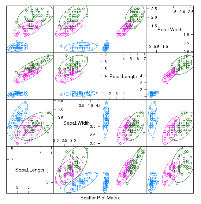
Scatterplot Matrix of Iris Data in R
We can also look at box and whisker plots of each input variable again, but this time broken down into separate plots for each class. This can help to tease out obvious linear separations between the classes.
|
1
2
|
# box and whisker plots for each attribute
featurePlot(x=x, y=y, plot=“box”)
|
This is useful to see that there are clearly different distributions of the attributes for each class value.
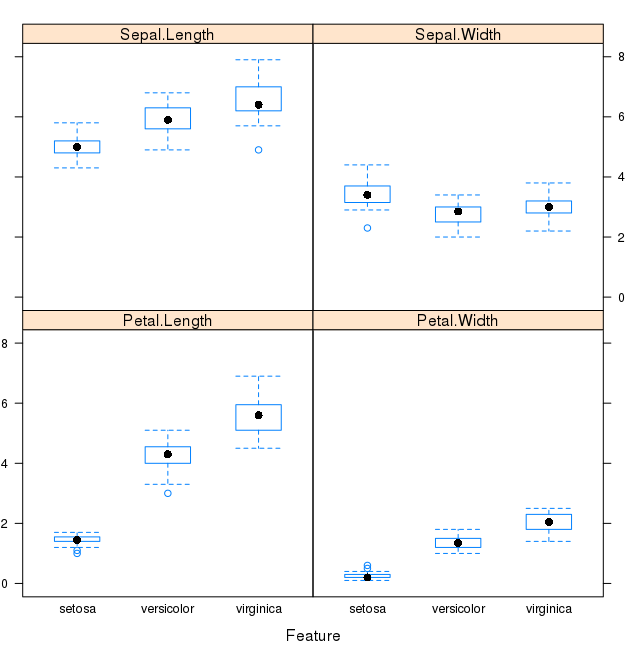
Box and Whisker Plot of Iris data by Class Value
Next we can get an idea of the distribution of each attribute, again like the box and whisker plots, broken down by class value. Sometimes histograms are good for this, but in this case we will use some probability density plots to give nice smooth lines for each distribution.
|
1
2
3
|
# density plots for each attribute by class value
scales <– list(x=list(relation=“free”), y=list(relation=“free”))
featurePlot(x=x, y=y, plot=“density”, scales=scales)
|
Like he boxplots, we can see the difference in distribution of each attribute by class value. We can also see the Gaussian-like distribution (bell curve) of each attribute.
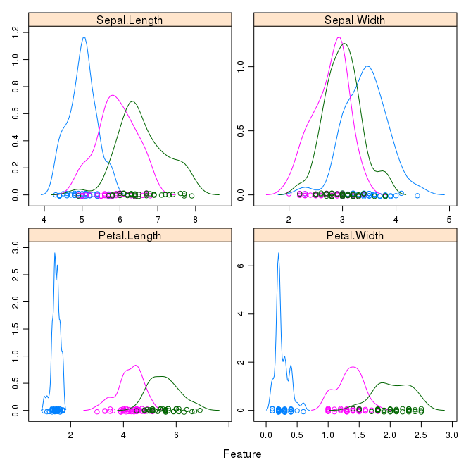
Density Plots of Iris Data By Class Value
5. Evaluate Some Algorithms
Now it is time to create some models of the data and estimate their accuracy on unseen data.
Here is what we are going to cover in this step:
- Set-up the test harness to use 10-fold cross validation.
- Build 5 different models to predict species from flower measurements
- Select the best model.
5.1 Test Harness
We will 10-fold crossvalidation to estimate accuracy.
This will split our dataset into 10 parts, train in 9 and test on 1 and release for all combinations of train-test splits. We will also repeat the process 3 times for each algorithm with different splits of the data into 10 groups, in an effort to get a more accurate estimate.
|
1
2
3
|
# Run algorithms using 10-fold cross validation
control <– trainControl(method=“cv”, number=10)
metric <– “Accuracy”
|
We are using the metric of “Accuracy” to evaluate models. This is a ratio of the number of correctly predicted instances in divided by the total number of instances in the dataset multiplied by 100 to give a percentage (e.g. 95% accurate). We will be using the metricvariable when we run build and evaluate each model next.
5.2 Build Models
We don’t know which algorithms would be good on this problem or what configurations to use. We get an idea from the plots that some of the classes are partially linearly separable in some dimensions, so we are expecting generally good results.
Let’s evaluate 5 different algorithms:
- Linear Discriminant Analysis (LDA)
- Classification and Regression Trees (CART).
- k-Nearest Neighbors (kNN).
- Support Vector Machines (SVM) with a linear kernel.
- Random Forest (RF)
This is a good mixture of simple linear (LDA), nonlinear (CART, kNN) and complex nonlinear methods (SVM, RF). We reset the random number seed before reach run to ensure that the evaluation of each algorithm is performed using exactly the same data splits. It ensures the results are directly comparable.
Let’s build our five models:
|
1
2
3
4
5
6
7
8
9
10
11
12
13
14
15
16
17
|
# a) linear algorithms
set.seed(7)
fit.lda <– train(Species~., data=dataset, method=“lda”, metric=metric, trControl=control)
# b) nonlinear algorithms
# CART
set.seed(7)
fit.cart <– train(Species~., data=dataset, method=“rpart”, metric=metric, trControl=control)
# kNN
set.seed(7)
fit.knn <– train(Species~., data=dataset, method=“knn”, metric=metric, trControl=control)
# c) advanced algorithms
# SVM
set.seed(7)
fit.svm <– train(Species~., data=dataset, method=“svmRadial”, metric=metric, trControl=control)
# Random Forest
set.seed(7)
fit.rf <– train(Species~., data=dataset, method=“rf”, metric=metric, trControl=control)
|
Caret does support the configuration and tuning of the configuration of each model, but we are not going to cover that in this tutorial.
5.3 Select Best Model
We now have 5 models and accuracy estimations for each. We need to compare the models to each other and select the most accurate.
We can report on the accuracy of each model by first creating a list of the created models and using the summary function.
|
1
2
3
|
# summarize accuracy of models
results <– resamples(list(lda=fit.lda, cart=fit.cart, knn=fit.knn, svm=fit.svm, rf=fit.rf))
summary(results)
|
We can see the accuracy of each classifier and also other metrics like Kappa:
|
1
2
3
4
5
6
7
8
9
10
11
12
13
14
15
16
17
18
|
Models: lda, cart, knn, svm, rf
Number of resamples: 10
Accuracy
Min. 1st Qu. Median Mean 3rd Qu. Max. NA’s
lda 0.9167 0.9375 1.0000 0.9750 1 1 0
cart 0.8333 0.9167 0.9167 0.9417 1 1 0
knn 0.8333 0.9167 1.0000 0.9583 1 1 0
svm 0.8333 0.9167 0.9167 0.9417 1 1 0
rf 0.8333 0.9167 0.9583 0.9500 1 1 0
Kappa
Min. 1st Qu. Median Mean 3rd Qu. Max. NA’s
lda 0.875 0.9062 1.0000 0.9625 1 1 0
cart 0.750 0.8750 0.8750 0.9125 1 1 0
knn 0.750 0.8750 1.0000 0.9375 1 1 0
svm 0.750 0.8750 0.8750 0.9125 1 1 0
rf 0.750 0.8750 0.9375 0.9250 1 1 0
|
We can also create a plot of the model evaluation results and compare the spread and the mean accuracy of each model. There is a population of accuracy measures for each algorithm because each algorithm was evaluated 10 times (10 fold cross validation).
|
1
2
|
# compare accuracy of models
dotplot(results)
|
We can see that the most accurate model in this case was LDA:
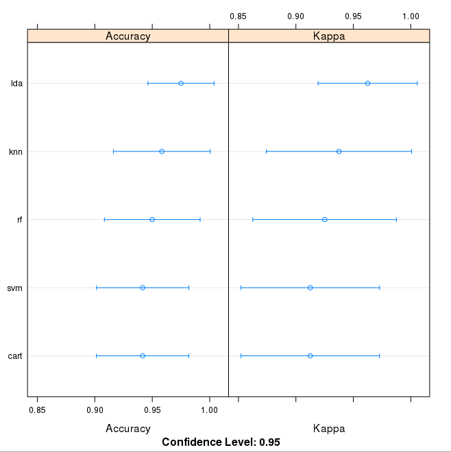
Comparison of Machine Learning Algorithms on Iris Dataset in R
The results for just the LDA model can be summarized.
|
1
2
|
# summarize Best Model
print(fit.lda)
|
This gives a nice summary of what was used to train the model and the mean and standard deviation (SD) accuracy achieved, specifically 97.5% accuracy +/- 4%
|
1
2
3
4
5
6
7
8
9
10
11
12
13
|
Linear Discriminant Analysis
120 samples
4 predictor
3 classes: ‘setosa’, ‘versicolor’, ‘virginica’
No pre-processing
Resampling: Cross-Validated (10 fold)
Summary of sample sizes: 108, 108, 108, 108, 108, 108, …
Resampling results
Accuracy Kappa Accuracy SD Kappa SD
0.975 0.9625 0.04025382 0.06038074
|
6. Make Predictions
The LDA was the most accurate model. Now we want to get an idea of the accuracy of the model on our validation set.
This will give us an independent final check on the accuracy of the best model. It is valuable to keep a validation set just in case you made a slip during such as overfitting to the training set or a data leak. Both will result in an overly optimistic result.
We can run the LDA model directly on the validation set and summarize the results in a confusion matrix.
|
1
2
3
|
# estimate skill of LDA on the validation dataset
predictions <– predict(fit.lda, validation)
confusionMatrix(predictions, validation$Species)
|
We can see that the accuracy is 100%. It was a small validation dataset (20%), but this result is within our expected margin of 97% +/-4% suggesting we may have an accurate and a reliably accurate model.
|
1
2
3
4
5
6
7
8
9
10
11
12
13
14
15
16
17
18
19
20
21
22
23
24
25
26
27
28
29
|
Confusion Matrix and Statistics
Reference
Prediction setosa versicolor virginica
setosa 10 0 0
versicolor 0 10 0
virginica 0 0 10
Overall Statistics
Accuracy : 1
95% CI : (0.8843, 1)
No Information Rate : 0.3333
P-Value [Acc > NIR] : 4.857e-15
Kappa : 1
Mcnemar’s Test P-Value : NA
Statistics by Class:
Class: setosa Class: versicolor Class: virginica
Sensitivity 1.0000 1.0000 1.0000
Specificity 1.0000 1.0000 1.0000
Pos Pred Value 1.0000 1.0000 1.0000
Neg Pred Value 1.0000 1.0000 1.0000
Prevalence 0.3333 0.3333 0.3333
Detection Rate 0.3333 0.3333 0.3333
Detection Prevalence 0.3333 0.3333 0.3333
Balanced Accuracy 1.0000 1.0000 1.0000
|
You Can Do Machine Learning in R
Work through the tutorial above. It will take you 5-to-10 minutes, max!
You do not need to understand everything. (at least not right now) Your goal is to run through the tutorial end-to-end and get a result. You do not need to understand everything on the first pass. List down your questions as you go. Make heavy use of the ?FunctionName help syntax in R to learn about all of the functions that you’re using.
You do not need to know how the algorithms work. It is important to know about the limitations and how to configure machine learning algorithms. But learning about algorithms can come later. You need to build up this algorithm knowledge slowly over a long period of time. Today, start off by getting comfortable with the platform.
You do not need to be an R programmer. The syntax of the R language can be confusing. Just like other languages, focus on function calls (e.g. function()) and assignments (e.g. a <- “b”). This will get you most of the way. You are a developer, you know how to pick up the basics of a language real fast. Just get started and dive into the details later.
You do not need to be a machine learning expert. You can learn about the benefits and limitations of various algorithms later, and there are plenty of posts that you can read later to brush up on the steps of a machine learning project and the importance of evaluating accuracy using cross validation.
What about other steps in a machine learning project. We did not cover all of the steps in a machine learning project because this is your first project and we need to focus on the key steps. Namely, loading data, looking at the data, evaluating some algorithms and making some predictions. In later tutorials we can look at other data preparation and result improvement tasks.
原创文章,作者:xsmile,如若转载,请注明出处:http://www.17bigdata.com/your-first-machine-learning-project-in-r-step-by-step-tutorial-and-template-for-future-projects/
注意:本文归作者所有,未经作者允许,不得转载