ComputeamovingaverageinSAS用SAS计算移动平均值

A common question on SAS discussion forums is how to compute a moving average in SAS. This article shows how to use PROC EXPAND and contains links to articles that use the DATA step or macros to compute moving averages in SAS.

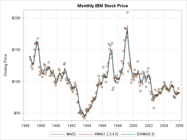In a previous post, I explained how to define a moving average and provided an example, which is shown here. The graph is a scatter plot of the monthly closing price for IBM stock over a 20-year period. The three curves are moving averages. The “MA” curve is a five-point (trailing) moving average. The “WMA” curve is a weighted moving average with weights 1 through 5. (When computing the weighted moving average at time t, the value y_thas weight 5, the value y_t-1 has weight 4, the value y_t-2 has weight 3, and so forth.) The “EWMA” curve is an exponentially weighted moving average with smoothing factor α = 0.3.

This article shows how to use the EXPAND procedure in SAS/ETS software to compute a simple moving average, a weighted moving average, and an exponentially weighted moving average in SAS. For an overview of PROC EXPAND and its many capabilities, I recommend reading the short paper “Stupid Human Tricks with PROC EXPAND” by David Cassell (2010).

Because not every SAS customer has a license for SAS/ETS software, there are links at the end of this article that show how to compute a simple moving average in SAS by using the DATA step.

Create an example time series

Before you can compute a moving average in SAS, you need data. The following call to PROC SORT creates an example time series with 233 observations. There are no missing values. The data are sorted by the time variable, T. The variable Y contains the monthly closing price of IBM stock during a 20-year period.

/* create example data: IBM stock price */
title "Monthly IBM Stock Price";
proc sort data=sashelp.stocks(where=(STOCK='IBM') rename=(Date=t Close=y)) 
          out=Series;
  by t;
run;

Compute a moving average in SAS by using PROC EXPAND

PROC EXPAND computes many kinds of moving averages and other rolling statistics, such as rolling standard deviations, correlations, and cumulative sums of squares.

In the procedure, the ID statement identifies the time variable, T. The data should be sorted by the ID variable. The CONVERT statement specifies the names of the input and output variables. The TRANSFORMOUT= option specifies the method and parameters that are used to compute the rolling statistics.

/* create three moving average curves */
proc expand data=Series out=out method=none;
   id t;
   convert y = MA   / transout=(movave 5);
   convert y = WMA  / transout=(movave(1 2 3 4 5)); 
   convert y = EWMA / transout=(ewma 0.3);
run;

The example uses three CONVERT statements:

• The first specifies that MA is an output variable that is computed as a (backward) moving average that uses five data values (k=5).
• The second CONVERT statement specifies that WMA is an output variable that is a weighted moving average. The weights are automatically standardized by the procedure, so the formula is WMA(t) = (5y_t + 4y_t-1 + 3y_t-2 + 2y_t-3 + 1y_t-4) / 15.
• The third CONVERT statement specifies that EWMA is an output variable that is an exponentially weighted moving average with parameter 0.3.

Notice the METHOD=NONE option on the PROC EXPAND statement. By default, the EXPAND procedure fits cubic spline curves to the nonmissing values of variables. The METHOD=NONE options ensures that the raw data points are used to compute the moving averages, rather than interpolated values.

Visualizing moving averages

An important use of a moving average is to overlay a curve on a scatter plot of the raw data. This enables you to visualize short-term trends in the data. The following call to PROC SGPOT creates the graph at the top of this article:

proc sgplot data=out cycleattrs;
   series x=t y=MA   / name='MA'   legendlabel="MA(5)";
   series x=t y=WMA  / name='WMA'  legendlabel="WMA(1,2,3,4,5)";
   series x=t y=EWMA / name='EWMA' legendlabel="EWMA(0.3)";
   scatter x=t y=y;
   keylegend 'MA' 'WMA' 'EWMA';
   xaxis display=(nolabel) grid;
   yaxis label="Closing Price" grid;
run;

To keep this article as simple as possible, I have not discussed how to handle missing data when computing moving averages. See the documentation for PROC EXPAND for various issues related to missing data. In particular, you can use the METHOD= option to specify how to interpolate missing values. You can also use transformation options to control how moving averages are defined for the first few data points.

Create a moving average in SAS by using the DATA step

If you do not have SAS/ETS software, the following references show how to use the SAS DATA step to compute simple moving averages by using the LAG function:

• The SAS Knowledge Base provides the article “Compute the moving average of a variable.”
• Premal Vora (2008) compares the DATA step to PROC EXPAND code in the paper “Easy Rolling Statistics with PROC EXPAND.”
• Ron Cody includes a SAS macro in several of his books. For example, Cody’s Collection of Popular SAS Programming Tasks and How to Tackle Them provides a macro named %moving_Ave. You can download the macro as part of the “Example Code and Data” for the book.

The DATA step, which is designed to handle one observation at a time, is not the best tool for time series computations, which naturally require multiple observations (lags and leads). In a future blog post, I will show how to write SAS/IML functions that compute simple, weighted, and exponentially weighted moving averages. The matrix language in PROC IML is easier to work with for computations that require accessing multiple time points.