聊聊样本采样技术

作者大可华东理工大学计算机应用技术博士

本人在腾讯/微信从事推荐系统相关工作，会将平时遇到的业务问题和相应的解决方案总结成公众号文章，感兴趣的可以关注本人公众号：泛函的范

在实际应用中经常会遇到类别不平衡问题，如

1）推荐系统中，曝光行为要远大于用户的点击行为，而点击行为又要远大于交易行为；
2）在欺诈交易检测中，欺诈交易订单是占总交易数量非常少的一部分的；
3）在工厂质量检测中，合格产品的数量是远大于不合格产品的；
4）信用卡的征信中，信用正常的用户是远多于信用有风险的用户的。

这里的“不均衡”指的是数据集中各个类别的样本数量差异较大（如某些类别样本数是其他类别的成百上千倍）。由于传统机器学习算法的损失函数（比交叉熵、均方误差）都是假设样本具有相同权重的（即每个样本被错分的对模型的惩罚是相同的），这导致如果数据集中某类样本过少，该类对模型的惩罚力度不够，模型就会”轻视”这类样本。

我们以二分类问题为例，假设正样本数量远少于负样本数量（如正负样本比为1:100），此时如果模型将所有样本全部判别为负类，如：

所有样本的预测结果为： $y_{pred}=0.0099=\frac{1}{101}$
corssentropy loss为 $0.0555$
模型的准确率为 $99\%$

从这些指标来看，模型的效果很好的，但对于这个不平衡问题来说，其实模型的效果是不可用的，因为他完全不能区分正负样本。由此可见，在面对不平衡问题时，采用传统方法并不能有效解决。

本文总结了处理样本不平衡问题的主要方法，并结合在人工数据集的实验对比各方法的效果，且附上了对应的python实现代码。希望能帮大家加深对这些方法的理解和应用。

需要再说明一点：对于分类问题，模型学习的是数据类别的分界。每次训练过程相当于不断修正分界线。因此，重采样方法理论上会导致分界线受到分布改变的影响。但分界线一般处在分布边缘，影响并不会特别大。有时候重采样过多，对分界线的影响较大，反而会导致模型结果变差。所以一个好的重采样方法应该不是把类别样本数量固定成1:1，而是把这个比例当作一个超参数，针对不同数据集做出调整，来保证模型的有效性。

〇、数据&Baseline

在讲具体方法前，先要构造一个人工不平衡数据集，然后以常规方法在该数据集上的效果作为我们的baseline，方便我们对比后续各种方法的效果。

1、数据生成

我们采用sklearn.datasets.make_classification，正负样本比为5:95

from sklearn.datasets import make_classification
X, y = make_classification(n_samples=10000,
                           n_classes=2,
                           weights=[0.95, 0.05],
                           class_sep=1.2,
                           n_features=8,
                           n_informative=4,
                           n_redundant=1,
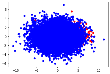
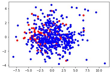
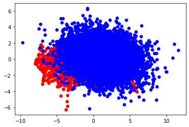
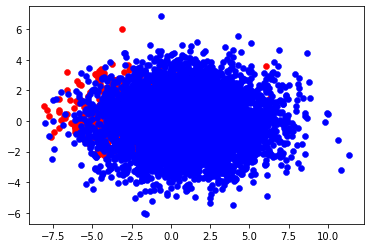
                           n_clusters_per_class=1)

然后采用PCA将数据降维到2维空间，可视化数据集的空间分布:

from sklearn.decomposition import PCA
def pca_draw(X, y): 
    pca = PCA(n_components=2)
    pca.fit(X)
    n_X = pca.transform(X)
    pos_X, neg_X = n_X[y==1], n_X[y==0]
    pos_X.shape, neg_X.shape
    plt.scatter(pos_X[:,0], pos_X[:,1], c='r', linewidths=0.5)
    plt.scatter(neg_X[:,0], neg_X[:,1], c='b', linewidths=0.5)

pca_draw(X, y)
print('n_pos = %d, n_neg=%d'%(np.sum(y==1), np.sum(y==0)))
# n_pos = 550, n_neg=9450

生成的数据中：正样本536个，负样本9464个。数据集在二维空间的分布如下：

2、训练-测试样本划分

将数据集随机按照7:3划分法成训练集和测试集：

trn_idx = np.array([1 if random.random()<0.7 else 0 for i in range(X.shape[0])])
trn_X = X[trn_idx==1]
trn_y = y[trn_idx==1]
tst_X = X[trn_idx==0]
tst_y = y[trn_idx==0]

3、评估方法

由于不平衡数据集中正、负样本差异较大，采用传统的正确率指标并不能有效反应模型效果。在实际业务中，往往对多数类（即负样本）更关注其准确性（precision），对于少数类（即正样本）则更关注其召回率（recall）。因此本文采用负样本precision和正样本recall来评估模型在不平衡数据集上的效果：

def evaluate(y_true, y_pred):
    pos_recall = np.sum(y_pred[y_true==1]>0.5)/np.sum(y_true==1)
    neg_precision = np.sum(y_true[y_pred<0.5]<0.5)/np.sum(y_pred<0.5)
    return pos_recall, neg_precision

4、Baseline

我们采用LogisticRegression在原始数据集上的效果来作为baseline：

from sklearn.model_selection import RepeatedKFold
from sklearn.model_selection import cross_val_score
from sklearn.linear_model import LogisticRegression
cv = RepeatedKFold(n_splits=5, n_repeats=3, random_state=1)

def lr_predict(trn_X, trn_y, tst_X, tst_y, class_weight=None):
    C_list = [0.001, 0.01, 0.1, 1, 10, 100]
    bst_c = C_list[0]
    bst_m = 0
    for c in C_list:
        model = LogisticRegression(C=c, class_weight=class_weight)
        scores = cross_val_score(model, trn_X, trn_y, scoring='roc_auc', cv=cv, n_jobs=-1)
        print('C = %.3f --> auc: %.5f (%.5f), bst: %.5f' % (c, np.mean(scores), np.std(scores), bst_m))
        if np.mean(scores)>bst_m:
            bst_c = c
            bst_m = np.mean(scores)
    model = LogisticRegression(C=bst_c, class_weight=class_weight)
    model.fit(trn_X, trn_y)

    tst_pred = model.predict_proba(tst_X)
    p_r, n_p = evaluate(tst_y, tst_pred[:,1])
    print('Precison on Majarity: %.3f, Recall on Minority: %.3f'%(n_p, p_r))

一、样本加权

在处理不平衡问题时，为了突出正样本的重要性，可以在损失函数中对样本进行加权。以LogisticRegression为例，原始损失函数为：

$L = - \sum_{j \in C}{\sum_{y_i=j}{ln(P(y_i=j|x_i;\Theta)}}$

其中$C$是类别的集合， $(x_i, y_i)$ 表示样本和对应的label。通过对不同类别的样本进行加权 $w_j$ （表示第$j$类的样本的权重），损失函数可以表示为：

$L_w = - \sum_{j\in C}{\sum_{y_i=j}{w_j ln(P(y_i=j|x_i;\Theta)}}$

有很多论文对如何确定样本权重的做了深入研究，感兴趣的读者可以进一步阅读参考文献先中的内容。在本文中，我们采用比较简单的方法来计算正、负类的权重：

$w_{pos} = \frac{|POS|}{|S|} \\ w_{neg} = \frac{|NEG|}{|S|}$

其中， $POS$ 和 $NEG$ 分别表示正、负样本集合， $S=POS \cup NEG$ 表示全部样本集。

最终加权的LR在测试集上的预测结果如下：

w_pos = np.sum(trn_y==0)/trn_y.shape[0]
w_neg = np.sum(trn_y==1)/trn_y.shape[0]

w_pos = 0.945, w_neg = 0.055

二、多数类样本下采样

多数类样本下采样方法主要是通过移除部分多数类样本来解决训练集中正负样本不平衡问题。由于删除了部分负样本，容易造成信息损失，可能会造成模型的准确度的下降。

1、随机下采样

随机下采样直接将训练集中负样本按照一定概率随机删除，从而达到正负样本的平衡

def random_undersampling(X, y, balanced_ratio=0.5):
    '''
        balanced_ratio = n_pos/n_neg
    '''
    ratio = (np.sum(y==1)/np.sum(y==0))/balanced_ratio
    n_under_sampling_idx = np.array([0 if y[i]==0 and random.random()>ratio else 1 for i in range(y.shape[0])])
    n_X = X[n_under_sampling_idx==1]
    n_y = y[n_under_sampling_idx==1]
    print('before: n_pos= %d, n_neg = %d'%(np.sum(y==1), np.sum(y==0)))
    print('after: n_pos= %d, n_neg = %d'%(np.sum(n_y==1), np.sum(n_y==0)))
    return n_X, n_y

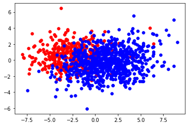
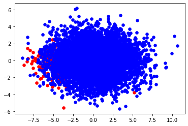
n_trn_X, n_trn_y = random_undersampling(trn_X, trn_y, balanced_ratio=0.5)
pca_draw(n_trn_X, n_trn_y)

'''
before: n_pos= 391, n_neg = 6672
after: n_pos= 391, n_neg = 748
'''

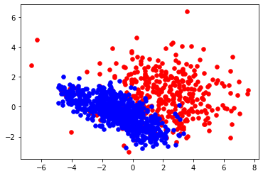
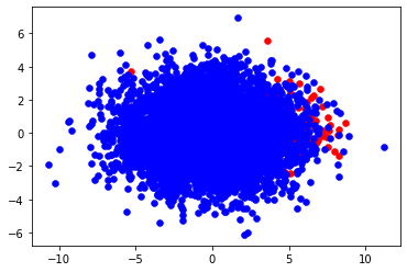
2、NearMiss

NearMiss是Man等人在2003年提出来的，其核心思想是：保留多数类中距离少数类中最近的k个样本的平均距离之和最小的点，其中k是超参数。

from sklearn.neighbors import DistanceMetric

def near_miss(X, y, k, balanced_ratio=0.5):
    pos = X[y==1]
    neg = X[y==0]

    n_sample = int(pos.shape[0]/balanced_ratio)

    dist = DistanceMetric.get_metric('euclidean')
    n_d = dist.pairwise(neg, pos)
    top_k_idx = n_d.argsort()[:,:k]
    dist_2_k_pos = np.mean([n_d[i][top_k_idx[i]] for i in range(trn_neg.shape[0])], axis=1)
    sampled_S = neg[dist_2_k_pos.argsort()[:n_sample]]

    n_X = np.vstack((sampled_S, pos))
    n_y = np.array([0]*sampled_S.shape[0] + [1]*pos.shape[0])
    print('before: n_pos= %d, n_neg = %d'%(np.sum(y==1), np.sum(y==0)))
    print('after: n_pos= %d, n_neg = %d'%(np.sum(n_y==1), np.sum(n_y==0)))
    return n_X, n_y

n_trn_X, n_trn_y =near_miss(trn_X, trn_y, k=3, balanced_ratio=0.5)
'''
before: n_pos= 391, n_neg = 6672
after: n_pos= 391, n_neg = 782
'''

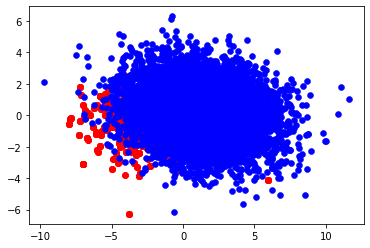
3、Condense Nearest Neighbor（CNN）

本方法是Hart在2006年提出来的，其核心思想：从整个样本集S中筛选出子集U，使得S中的每个样本的最近邻样本与它自己具有相同标签。

具体流程可以概述为：

从S中随机选择一个样本p，并加入到U中：U={p}
在S-U中扫描样本，将第一个满足条件（其在U中最近的样本与它自己具有不同类别）的样本p加入到U中
持续运行第二步，直到U不在增加

from sklearn.neighbors import DistanceMetric

def condensed_nn(X, y):
    S_fea = X
    S_idx = [i for i in range(1, X.shape[0])]
    U = [0]

    dist = DistanceMetric.get_metric('euclidean')

    for i in range(X.shape[0]):
        prev_len_u = len(U)

        n_s_idx = np.array(S_idx)
        n_u_idx = np.array(U)
        n_d = dist.pairwise(S_fea[n_s_idx], S_fea[n_u_idx])

        for i in range(n_d.shape[0]):
            nearest_u_idx = n_u_idx[n_d[i].argsort()[0]]
            p_idx = n_s_idx[i]
            if y[nearest_u_idx] != y[p_idx]:
                U.append(p_idx)
                S_idx.remove(p_idx)
                break
        if prev_len_u == len(U):
            break

    n_U = np.array(list(set(U + [i for i in range(y.shape[0]) if y[i]==1])))
    n_X, n_y = X[np.array(n_U)], y[np.array(n_U)]
    print('before: n_pos= %d, n_neg = %d'%(np.sum(y==1), np.sum(y==0)))
    print('after: n_pos= %d, n_neg = %d'%(np.sum(n_y==1), np.sum(n_y==0)))
    return n_X, n_y

n_trn_X, n_trn_y = condensed_nn(trn_X, trn_y)
'''
before: n_pos= 391, n_neg = 6672
after: n_pos= 391, n_neg = 557
'''

4、Edited Nearest Neighbor（ENN）

本方法是Wilson在1972年提出的，其核心思想是：通过移除那些类别标签与其k近邻的大多数标签不同的多数类样本，来对多数类进行下采样

def edited_nn(X, y, k, isthrd=True, islog=True):
    thrd = 1 if not isthrd else k/2
    neg = X[y==0]
    dist = DistanceMetric.get_metric('euclidean')
    n_d = dist.pairwise(neg, X)
    top_k_idx = n_d.argsort()[:,:k+1]
    top_k_label = np.array([y[top_k_idx[i]] for i in range(top_k_idx.shape[0])])
    n_X = np.vstack((neg[np.sum(top_k_label, axis=1)<thrd], X[y==1]))
    n_y = np.array([0]*np.sum(np.sum(top_k_label, axis=1)<thrd) + [1]*np.sum(y==1))

    print('before: n_pos= %d, n_neg = %d'%(np.sum(y==1), np.sum(y==0)))
    print('after: n_pos= %d, n_neg = %d'%(np.sum(n_y==1), np.sum(n_y==0)))
    return n_X, n_y

n_trn_X, n_trn_y = edited_nn(trn_X, trn_y, k=15)
'''
before: n_pos= 391, n_neg = 6672
after: n_pos= 391, n_neg = 5850
'''

5、Tomek Link Removal

本方法是Tomek在1976年提出的，其核心思想是：如果一对最近邻的样本分别属于不同类别，则将该样本对称为是Tomek link。可以通过移除Tomek link中的多数类样本来实现对多数类样本的下采样。

def tomek_link_rm(X, y):
    dist = DistanceMetric.get_metric('euclidean')
    n_d = dist.pairwise(X, X)
    top_k_idx = n_d.argsort()[:,:2]

    tomek_link_idx = [[top_k_idx[i][0], top_k_idx[i][1]] for i in range(top_k_idx.shape[0]) if np.sum(y[top_k_idx[i]])==1]

    rm_pos_idx = [idx for idx in set([pair[0] for pair in tomek_link_idx] + [pair[1] for pair in tomek_link_idx]) if y[idx]==0]
    print('tomek_link pairs = %d, removed pos samples = %d'%(len(tomek_link_idx), len(rm_pos_idx)))
    retained_flag = np.array([1]*X.shape[0])
    retained_flag[np.array(rm_pos_idx)]=0

    n_X = X[retained_flag==1]
    n_y = y[retained_flag==1]

    print('before: n_pos= %d, n_neg = %d'%(np.sum(y==1), np.sum(y==0)))
    print('after: n_pos= %d, n_neg = %d'%(np.sum(n_y==1), np.sum(n_y==0)))
    return n_trn_X, n_trn_y

n_trn_X, n_trn_y = tomek_link_rm(X=trn_X, y=trn_y)
'''
tomek_link pairs = 145, removed pos samples = 116
before: n_pos= 391, n_neg = 6672
after: n_pos= 391, n_neg = 6556
'''

三、少数类样本上采样

平衡样本的另一种方式是对少数类样本进行上采样。但上采样方法额外增加了正样本，容易引入噪声，可能会导致模型对少数类样本过拟合。

本节主要介绍三种常用的上采样方法：1）随机上采样；2）SMOTE；3）Borderline-SMOTE。

1、随机上采样

核心思想是：通过随机对少数类样本进行复制，缓解样本间的不平衡。但随机上采样是通过简单复制样本的策略来增加少数类样本，这样容易产生模型过拟合的问题。

def random_oversampling(X, y, balanced_ratio=0.5):
    '''
        balanced_ratio = n_pos/n_neg
    '''
    r = np.sum(y==1)/np.sum(y==0)
    if r > balanced_ratio:
        return X, y

    n_over_pos = int(np.sum(y==0)*balanced_ratio - np.sum(y==1))
    pos_idx = [i for i in range(y.shape[0]) if y[i]==1]
    sampled_idx = np.random.choice(pos_idx, n_over_pos)
    n_X = np.vstack((X, X[sampled_idx]))
    n_y = np.hstack((y, y[sampled_idx]))

    print('before: n_pos = %d, n_neg = %d'%(np.sum(y==1), np.sum(y==0)))
    print('after: n_pos = %d, n_neg = %d'%(np.sum(n_y==1), np.sum(n_y==0)))
    return n_X, n_y

n_trn_X, n_trn_y = random_oversampling(X=trn_X, y=trn_y, balanced_ratio=0.5)
'''
before: n_pos = 391, n_neg = 6672
after: n_pos = 3336, n_neg = 6672
'''

2、SMOTE

SMOTE（Synthetic Minority Oversampling Technique）的基本思想是对少数类样本进行分析并生成人工合成新样本，具体如下图所示：

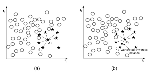
SMOTE步骤如下：

计算样本 $x_i$ 的最近 $k$ 个样本
随机从 $k$ 个近邻样本中选出一个样本 $x_i^j$ ，并在 $x_i$ 和 $x_i^j$ 的连线上随机生产样本 $\hat{x}_i^j$
重复步骤2，知道生成满足数量的人工样本

我们可以直接采用imblearn包中的SMOTE算法来对样本进行上采样：

from imblearn.over_sampling import SMOTE

def smote(X, y, balanced_ratio=0.5):
    n_pos = int(np.sum(y==0)*0.5)
    model = SMOTE(sampling_strategy={1:n_pos})
    n_X, n_y = model.fit_resample(X, y)
    print('before: n_pos = %d, n_neg = %d'%(np.sum(y==1), np.sum(y==0)))
    print('after: n_pos = %d, n_neg = %d'%(np.sum(n_y==1), np.sum(n_y==0)))
    return n_X, n_y

n_trn_X, n_trn_y = smote(trn_X, trn_y, balanced_ratio=0.25)
'''
before: n_pos = 391, n_neg = 6672
after: n_pos = 3336, n_neg = 6672
'''

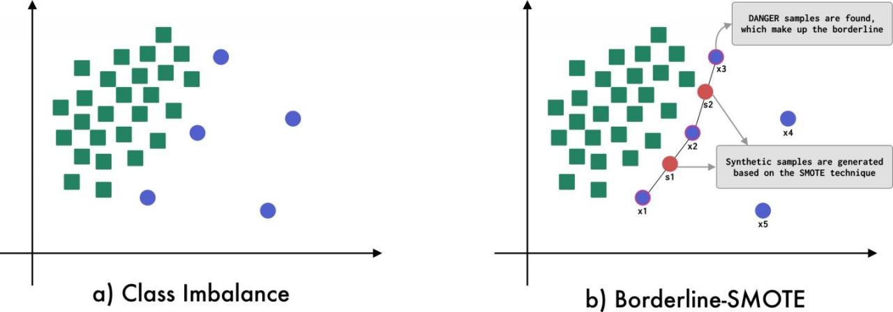
3、Borderline-SMOTE

Borderline SMOTE是在SMOTE基础上改进的少数类样本上采样算法。不同于SMOTE算法，Borderline SMOTE仅使用边界上的少数类样本来生成新的样本，从而改善样本的类别分布（因此，Borderline SMOTE又被称为SVM-SMOTE）。 Borderline SMOTE在采样过程中将少数类样本分为3类：NOISE、SAFE和DANGER。

对于每个少数类样本$x$，具体说明如下

从所有样本集合 $S$ 中计算 $x$ 的 $k$ 个最近邻样本，记为 $M$
求 $M$ 与所有多数类样本的交集，记为 $M'= M \cap S_N$
判断样本 $x$ 的类型：
如果 $|M| = |M'|$ ，则将 $x$ 记为NOISY
如果 $0 \leq |M'| \leq |M|/2$ ，则将 $x$ 记为SAFE
如果 $|M|/2 \leq |M'| \leq |M|$ ，则将 $x$ 记为DANGER

最后，对于所有标记为DANGER的正样本，采用SMOTE算法来生成人工样本。

我们同样可以采用imblearn的BorderlineSMOTE方法来对少数类样本进行上采样：

from imblearn.over_sampling import BorderlineSMOTE

def borderline_smote(X, y, balanced_ratio=0.5):
    n_pos = int(np.sum(y==0)*0.5)
    model = BorderlineSMOTE(sampling_strategy={1:n_pos})
    n_X, n_y = model.fit_resample(X, y)
    print('before: n_pos = %d, n_neg = %d'%(np.sum(y==1), np.sum(y==0)))
    print('after: n_pos = %d, n_neg = %d'%(np.sum(n_y==1), np.sum(n_y==0)))
    return n_X, n_y

n_trn_X, n_trn_y = borderline_smote(trn_X, trn_y, balanced_ratio=0.25)
'''
before: n_pos = 391, n_neg = 6672
after: n_pos = 3336, n_neg = 6672
'''

四、下采样 & 上采样

在对不平衡数据集进行处理时，采用对多数类样本下采样的同时，对少数类样本进行上采样的效果要优于对单方面样本的处理。

本节介绍两种常用的混合采样方式：1）SMOTE+Tomek Link Removal；2) SMOTE+ENN

1、SMOTE + Tomek link removal

def combine_smote_tomek(X, y, balanced_ratio):
    # 采用Tomek Link Removal方法对多数类样本进行下采样
    n_X, n_y = tomek_link_rm(X, y)
    # 采用bordline SMOTE方法来对正样本上采样
    n_X, n_y = borderline_smote(n_X, n_y, balanced_ratio=balanced_ratio)
    print('before: n_pos = %d, n_neg = %d'%(np.sum(y==1), np.sum(y==0)))
    print('after: n_pos = %d, n_neg = %d'%(np.sum(n_y==1), np.sum(n_y==0)))
    return n_X, n_y

n_trn_X, n_trn_y = combine_smote_tomek(trn_X, trn_y, balanced_ratio=0.25)
'''
before: n_pos= 391, n_neg = 6672
after: n_pos = 3336, n_neg = 6672
'''

2、SMOTE + ENN

def combine_enn(X, y, k, balanced_ratio):
    # 采用Tomek Link Removal方法对多数类样本进行下采样
    n_X, n_y = edited_nn(X, y, k)
    # 采用bordline SMOTE方法来对正样本上采样
    n_X, n_y = borderline_smote(n_X, n_y, balanced_ratio=balanced_ratio)
    print('before: n_pos = %d, n_neg = %d'%(np.sum(y==1), np.sum(y==0)))
    print('after: n_pos = %d, n_neg = %d'%(np.sum(n_y==1), np.sum(n_y==0)))
    return n_X, n_y

n_trn_X, n_trn_y = combine_enn(trn_X, trn_y, k=7, balanced_ratio=0.25)
'''
before: n_pos= 391, n_neg = 6672
after: n_pos = 3143, n_neg = 6287
'''

五、集成方法

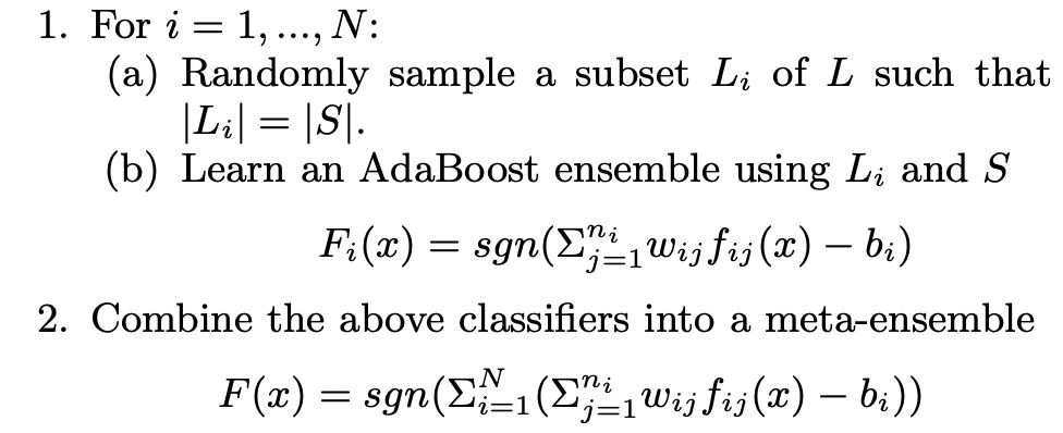
1、EasyEnsemble

EasyEnsemble算法是通过对多数类样本进行多次重采样，构造平衡多组平衡数据集，来训练若干个分类器进行集成学习。算法的具体步骤如下：

from sklearn.ensemble import GradientBoostingClassifier, RandomForestClassifier
def EasyEnsemble(trn_X, trn_y, tst_X, tst_y, clf, n_iter):
    num_pos = np.sum(trn_y)
    trn_pos = trn_X[trn_y==1]
    trn_neg = trn_X[trn_y==0]
    neg_idx = list(range(trn_neg.shape[0]))

    tst_pred = np.empty((tst_X.shape[0], n_iter))
    trn_pred = np.empty((trn_X.shape[0], n_iter))

    for i in range(n_iter):
        classifier = clf()
        # Sample the same number of negative cases as positive cases
        # neg_sample = trn_neg.sample(num_pos, random_state = i)
        sampled_neg_idx = np.random.choice(neg_idx, num_pos)
        neg_sample = trn_neg[sampled_neg_idx]
        x_sub = np.vstack((neg_sample, trn_pos))
        y_sub = np.array([0]*neg_sample.shape[0] + [1]*trn_pos.shape[0])

        # Fit the classifier to the balanced dataset
        classifier.fit(x_sub, y_sub)
        pred = classifier.predict_proba(tst_X)[:,1]
        tst_pred[:, i] = pred

    # Average all the test predictions
    ensemble_pred = np.mean(tst_pred, axis = 1)
    p_r, n_p = evaluate(tst_y, ensemble_pred)
    print('[%s] Precison on Majarity: %.3f, Recall on Minority: %.3f'%(clf.__name__, n_p, p_r))

我们可以分别采用如下三种分类器作为Emsemble算法的基分类器：

EasyEnsemble(trn_X, trn_y, tst_X, tst_y, clf=LogisticRegression, n_iter=20)
EasyEnsemble(trn_X, trn_y, tst_X, tst_y, clf=GradientBoostingClassifier, n_iter=20)
EasyEnsemble(trn_X, trn_y, tst_X, tst_y, clf=RandomForestClassifier, n_iter=20)

2、BalanceCascade

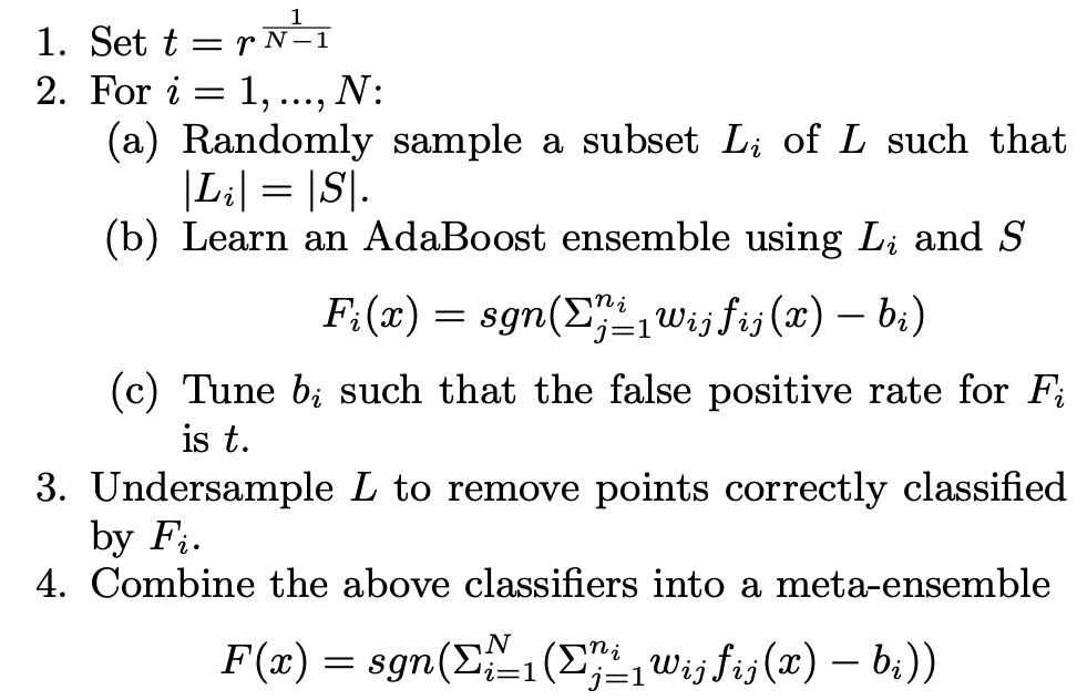
BalanceCascade算法与EasyEnsemble算法相似，只不过后者在样本采样时认为每次采样都是相互独立的（负样本每次具有相同概率被选中）。在BalanceCascade中，在每一轮训练后使用该分类器对全体多数类进行预测，将所有判断正确的类（数量=负样本总数×(1−FP)数量=负样本总数×(1−FP)）删除，然后进入下一轮迭代继续降低多数类数量。算法具体步骤如下：

def BalanceCascade(trn_X, trn_y, tst_X, tst_y, clf, n_iter):
    neg_num = np.sum(trn_y == 0)
    pos_num = np.sum(trn_y == 1)
    neg_idx = np.argwhere(trn_y == 0).reshape(neg_num, )
    pos_idx = np.argwhere(trn_y == 1).reshape(pos_num, )
    pos_trn = trn_X[pos_idx]

    FP = pow(pos_num/neg_num, 1/(n_iter-1))
    classifiers = {} 
    thresholds = {} 
    tst_prob = np.empty((tst_X.shape[0], n_iter))
    for i in range(n_iter):
        classifiers[i] = clf()
        neg_trn_idx = np.random.permutation(neg_idx)[:pos_num]
        neg_trn = trn_X[neg_trn_idx]
        sub_X = np.vstack((pos_trn, neg_trn))
        sub_y = np.array([1]*pos_trn.shape[0] + [0]*neg_trn.shape[0])
        classifiers[i].fit(sub_X, sub_y)
        trn_pred = classifiers[i].predict_proba(trn_X[neg_idx])[:,1]

        thresholds[i] = np.sort(trn_pred)[int(neg_idx.shape[0]*(1-FP))]
        neg_idx = np.argwhere(trn_pred >= thresholds[i]).reshape(-1, )
        tst_prob[:,i] = classifiers[i].predict_proba(tst_X)[:,1] + thresholds[i]

    ensemble_pred = np.average(tst_prob, axis=1)
    p_r, n_p = evaluate(tst_y, ensemble_pred)
    print('[%s] Precison on Majarity: %.3f, Recall on Minority: %.3f'%(clf.__name__, n_p, p_r))

我们可以分别采用如下三种分类器作为Emsemble算法的基分类器：

BalanceCascade(trn_X, trn_y, tst_X, tst_y, clf=LogisticRegression, n_iter=20)
BalanceCascade(trn_X, trn_y, tst_X, tst_y, clf=GradientBoostingClassifier, n_iter=20)
BalanceCascade(trn_X, trn_y, tst_X, tst_y, clf=RandomForestClassifier, n_iter=20)

总结

本文总结了在处理不平衡问的的常用方法，所涉及到的算法在人工数据集上的实验结果如下表所示：

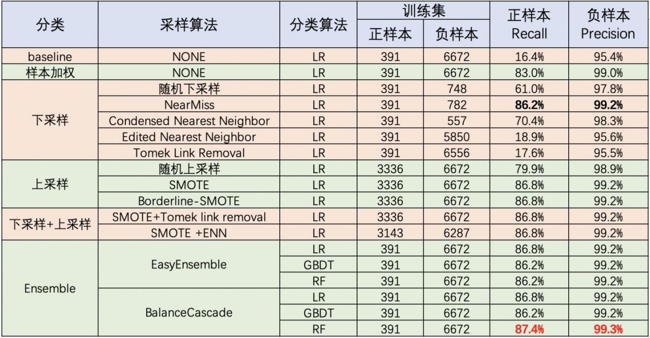
从实验结果可以看出：

LR在对于不平衡数据的处理效果并不好：倾向于将大多数样本判别为负样本，从而导致少数类样本的召回率只有16.4%；
总的来看，Ensemble方法的效果在处理不平衡问题生效果最好。但集成方法需要重复训练多个子分类器，效率相对较低；
对样本进行加权后的LR相比于原始LR在正样本召回和负样本准确率上均有显著提升；
在下采样方法中，NearMiss效果要优于其他下采样方法；
上采样方法中，SMOTE和Borderline-SMOTE要明显好于随机上采样。

综合考虑性能和效率，样本加权是个比较不错的选择。

参考文献

[1]. sklearn: https://scikit-learn.org/stable/

[2]. imblearn: https://imbalanced-learn.org/

[3]. Adaptive Weight Optimization for Classification of Imbalanced Data

[4]. Inderjeet Mani and I Zhang. knn approach to unbalanced data distributions: a case study involving information extraction. In Proceedings of workshop on learning from imbalanced datasets, 2003.

[5]. P. Hart. The condensed nearest neighbor rule. IEEE Transactions on Information Theory, 14(3):515–516, September 2006.

[6]. Dennis L Wilson. Asymptotic properties of nearest neighbor rules using edited data. IEEE Transactions on Systems, Man, and Cybernetics, (3):408–421, 1972.

[7]. Ivan Tomek. Two modifications of cnn. IEEE Transactions on Systems, Man and Cybernetics, 6:769–772, 1976.

[8]. Nitesh V. Chawla, Kevin W. Bowyer, Lawrence O. Hall, and W. Philip Kegelmeyer. Smote: synthetic minority over-sampling technique. Journal of artificial intelligence research, 16:321–357, 2002.

[9]. Hui Han, Wen-Yuan Wang, and Bing-Huan Mao. Borderline-smote: a new over-sampling method in imbalanced data sets learning. In International Conference on Intelligent Computing, pages 878–887. Springer, 2005.

[10]. Xu-Ying Liu, Jianxin Wu, and Zhi-Hua Zhou. Exploratory undersampling for class-imbalance learning. IEEE Transactions on Systems, Man, and Cybernetics, Part B (Cybernetics), 39(2):539–550, 2009.

本文来自zhihu，观点不代表一起大数据-技术文章心得立场，如若转载，请注明出处：https://zhuanlan.zhihu.com/p/383654750

更多内容请访问：IT源点

注意：本文归作者所有，未经作者允许，不得转载